


Figure 1.
Support vector machine.
Machine learning (ML) techniques are being increasingly applied to financial markets for analyzing trends and predicting stock prices. In this study, we compared the price prediction and profit-making performance of various ML algorithms embedded into stock trading strategies. The dataset comprised daily data from the CSI 300 Index of the China stock market spanning approximately 17 years (2006–2023). We incorporated investor sentiment indicators and relevant financial elements as features. Our trained models included support vector machines (SVMs), logistic regression, and random forest. The results show that the SVM model outperforms the others, achieving an impressive 60.52% excess return in backtesting. Furthermore, our research compared standard prediction models (such as LASSO and LSTM) with the proposed approach, providing valuable insights for users selecting ML algorithms in quantitative trading strategies. Ultimately, this work serves as a foundation for informed algorithm choice in future financial applications.
Citation: Haoyu Wang, Dejun Xie. Optimal profit-making strategies in stock market with algorithmic trading[J]. Quantitative Finance and Economics, 2024, 8(3): 546-572. doi: 10.3934/QFE.2024021
| [1] | Keyue Yan, Ying Li . Machine learning-based analysis of volatility quantitative investment strategies for American financial stocks. Quantitative Finance and Economics, 2024, 8(2): 364-386. doi: 10.3934/QFE.2024014 |
| [2] | Yimeng Wang, Keyue Yan . Machine learning-based quantitative trading strategies across different time intervals in the American market. Quantitative Finance and Economics, 2023, 7(4): 569-594. doi: 10.3934/QFE.2023028 |
| [3] | Andrey Kudryavtsev . Absolute Stock Returns and Trading Volumes: Psychological Insights. Quantitative Finance and Economics, 2017, 1(2): 186-204. doi: 10.3934/QFE.2017.2.186 |
| [4] | Mustafa Tevfik Kartal, Özer Depren, Serpil Kılıç Depren . The determinants of main stock exchange index changes in emerging countries: evidence from Turkey in COVID-19 pandemic age. Quantitative Finance and Economics, 2020, 4(4): 526-541. doi: 10.3934/QFE.2020025 |
| [5] | Samuel Kwaku Agyei, Ahmed Bossman . Investor sentiment and the interdependence structure of GIIPS stock market returns: A multiscale approach. Quantitative Finance and Economics, 2023, 7(1): 87-116. doi: 10.3934/QFE.2023005 |
| [6] | Diogo Matos, Luís Pacheco, Júlio Lobão . Availability heuristic and reversals following large stock price changes: evidence from the FTSE 100. Quantitative Finance and Economics, 2022, 6(1): 54-82. doi: 10.3934/QFE.2022003 |
| [7] | Wenhao Chen, Kinkeung Lai, Yi Cai . Topic generation for Chinese stocks: a cognitively motivated topic modelingmethod using social media data. Quantitative Finance and Economics, 2018, 2(2): 279-293. doi: 10.3934/QFE.2018.2.279 |
| [8] | Wenhui Li, Normaziah Mohd Nor, Hisham M, Feng Min . Volatility conditions and the weekend effect of long-short anomalies: Evidence from the US stock market. Quantitative Finance and Economics, 2023, 7(2): 337-355. doi: 10.3934/QFE.2023016 |
| [9] | Chiao Yi Chang, Fu Shuen Shie, Shu Ling Yang . The relationship between herding behavior and firm size before and after the elimination of short-sale price restrictions. Quantitative Finance and Economics, 2019, 3(3): 526-549. doi: 10.3934/QFE.2019.3.526 |
| [10] | Emmanuel Assifuah-Nunoo, Peterson Owusu Junior, Anokye Mohammed Adam, Ahmed Bossman . Assessing the safe haven properties of oil in African stock markets amid the COVID-19 pandemic: a quantile regression analysis. Quantitative Finance and Economics, 2022, 6(2): 244-269. doi: 10.3934/QFE.2022011 |
Machine learning (ML) techniques are being increasingly applied to financial markets for analyzing trends and predicting stock prices. In this study, we compared the price prediction and profit-making performance of various ML algorithms embedded into stock trading strategies. The dataset comprised daily data from the CSI 300 Index of the China stock market spanning approximately 17 years (2006–2023). We incorporated investor sentiment indicators and relevant financial elements as features. Our trained models included support vector machines (SVMs), logistic regression, and random forest. The results show that the SVM model outperforms the others, achieving an impressive 60.52% excess return in backtesting. Furthermore, our research compared standard prediction models (such as LASSO and LSTM) with the proposed approach, providing valuable insights for users selecting ML algorithms in quantitative trading strategies. Ultimately, this work serves as a foundation for informed algorithm choice in future financial applications.
Traditional research on asset pricing and price discovery has predominantly relied on economic knowledge, employing statistical methods and probability theory. However, as scholars delve deeper into stock trend forecasting and market dynamics continue to evolve, the limitations of traditional financial models become evident. The conventional financial models for stock trend prediction are basically in the realm of factor analysis, often involving hypothesis testing. Unfortunately, this approach falls short of accurately capturing real-world stock movements. The disparity between predicted trends and actual values remains substantial, leading to reduced prediction accuracy.
Machine learning algorithms have been suggested for better precision in the forecasting of stock behavior. By integrating the internal relationships within training data, these algorithms construct models capable of nonlinear processing and collaboration across multiple input features. Machine learning has already made significant strides in various fields including data mining, natural language processing, and pattern recognition. With the continuous accumulation of industry-specific data, organizations seek to leverage intelligent algorithms to extract valuable insights. In the context of stock price prediction, machine learning methods are supposed to yield high-precision models, guiding investors toward better decisions, risk reduction, and optimized returns.
While no universally optimal algorithm exists, certain methods excel in specific scenarios, achieving local optimality. Machine learning algorithms share this nuanced behavior. Scholars leverage extensive data and model tuning to demonstrate the efficacy of specific machine learning approaches in forecasting financial time series. In specific contexts, certain algorithms may outperform others. The financial industry boasts a wealth of historical data samples, ideal for systematic learning by machine learning algorithms. With numerous conditional variables related to risk premiums, the industry has cultivated a robust set of predictors. Notably, Green et al. (2013) identified 330 stock-level prediction signals, while Harvey et al. (2016) scrutinized 316 factors—encompassing firm characteristics and common elements—to elucidate stock return behavior. The crux lies in assessing the broader applicability of different machine learning algorithms across general financial time series prediction scenarios. Understanding the inherent advantages and disadvantages thereof is crucial.
There are hundreds of currently available stock-level predictive features, while macroeconomic predictive features for the overall market alone are in the dozens. Traditional economic approaches struggle when predicted values closely align with observed values or exhibit strong similarity. Machine learning, with its variable selection and dimensionality reduction techniques, is well-suited for such complex prediction tasks. By reducing degrees of freedom and eliminating redundant variables, machine learning effectively addresses issues of endogeneity and correlation. Leveraging extensive raw macroeconomic data—including long time series and multi-dimensional features—provides robust training and testing sets for the learning prediction models. Comparing various machine learning algorithms empirically is essential to identify the most applicable method for predicting asset prices in the capital market.
This study explores the behavioral perspective of the stock market, emphasizing the impact of investor sentiment and relevant financial and technical indicators. Employing empirical machine learning models, the study backtests a variety of investment strategies and provides implementable guidance for investors. More specifically, the study predicts the daily closing price movements of the CSI 300 index by combining investor sentiment analysis with technical indicators. Leveraging stock trading data from China's stock market data from January 2006 to December 2020, the study incorporates both financial and technical indicators into machine learning models for training, simulation, and testing. By comparing the profit performances of various strategies with the current CSI 300 index, the study generates accurate and comprehensive conclusions about the effectiveness of various machine learning models, thus providing hands-on guidance for algorithm trading of stocks.
Zweig (1973) defined investment sentiment as the difference between the true value of closed-end funds and the price expected by investors. Subsequently, De Long et al. (1990) conducted a study on the stock market and highlighted the presence of diverse voices within it. Reasonable investors, armed with available information, make informed judgments and avoid noise interference. In contrast, noise traders perceive these noises as valuable, influencing their investment decisions—this phenomenon is what we refer to as investor sentiment. Lee et al. (1991) proposed that the elusive quality such as the expected value of assets should be part of that sentiment. On a different note, Barberis et al. (1998), from both a psychological and mathematical perspective, argued that investor sentiment arises due to investors deviating from the subjective expected utility theory or irrationally applying Bayes' law when determining financial asset prices. They contended that investor sentiment is a cognitive process that significantly impacts investors' value judgments and perceptions. Furthermore, Baker and Stein (2004) asserted that inappropriate valuation of high-risk capital contributes to investor sentiment, leading to speculative behavior among market participants.
Investor sentiment, often rooted in market participants' biases, plays a crucial role in shaping financial outcomes. Yang and Li (2013) presented an asset pricing model that incorporates investor sentiment and information, and the results show that investor sentiment has a systematic and significant effect on asset prices. Rational periods of equilibrium prices drive asset prices toward rationality, and emotional periods cause asset prices to deviate from rationality. Yang and Zhou (2015) investigated the impact of investor trading behavior and investor sentiment on asset prices. They found that both investor trading behavior and investor sentiment have significant effects on excess returns. Meanwhile, the effect of investor trading behavior on excess returns is more significant than the effect of investor sentiment. The empirical results show that investor trading behavior and investor sentiment have a greater impact on the excess returns of small stocks than large stocks.
As to the relationship between investor sentiment and stock market volatility, the research remains inconclusive. However, researchers have broadly agreed that investors' psychological factors significantly influence the operational dynamics of securities trading, particularly impacting liquidity, yield, and market volatility. Current research predominantly centers on multifaceted and asymmetric effects of investor sentiment. For instance, Chau et al. (2016) explored sentiment effects in the US stock market, observing divergent investor reactions during market movements. While the overall stock market tends to exhibit a positive attitude, bear markets surprisingly witness more favorable stock performance than bull markets. Qiang and Shu-e (2009), building upon an enhanced noise trading theory model (De Long et al., 1990), delved into the subjective sentiment mechanisms of noise traders. They contended that investors' sentiment fluctuations exert a more substantial impact on stock prices than theoretically anticipated. Additionally, Zhang et al. (2021) found that text sentiment can effectively predict the volatility of the stock market, further confirming the impact of investor sentiment on financial markets.
Investor sentiment significantly impacts the average return of the market. Frugier (2016) confirmed that investor sentiment can be leveraged to construct profitable portfolios. Subsequently, Gu and Xu (2022) demonstrated that there is a two-way causal relationship between investor sentiment and market index: optimism or pessimism in investor sentiment affects the volatility of the CSI 300 Index, and an upward or downward movement of the index in return affects the state of investor sentiment. He et al. (2019) found that investor risk compensation (IRC) has a significant effect on stock market returns and this effect is moderated by investor sentiment. Current risk compensation has a positive effect on stock returns, while past risk compensation shows a negative effect on stock returns. Da et al. (2015) introduced the FEARS index, a novel measure of investor sentiment. His research indicated that the FEARS index predicts short-term reversals in returns, fluctuations in market volatility, and the flow of capital from the stock market to the bond market.
Balcilar et al. (2017) extended their investigation to the gold market. Their findings revealed that investor mindset exerts a greater influence on daily volatility than on daily returns. Specifically, investor sentiment can serve as a reflection of the volatility characteristics of safe-haven assets, providing a valuable theoretical foundation for risk management and option pricing. In a related study, Lin et al. (2018) delved into the impact of investor psychology on the dynamic pricing of commodities in both spot and futures commodity markets. They highlighted that, when positive signals abound in the market, several factors experience heightened levels of volatility: price fluctuations, arbitrage risk, and buying and selling costs. Interestingly, investors in the futures market often exhibit reluctance to leverage heterogeneous information at their disposal, thereby diminishing the role of the futures market as an information precursor and price discovery mechanism.
Machine learning has made significant strides in stock price prediction in recent years. Among the widely used methods, support vector machines (SVMs), logistic regression, and the random forest model stand out. SVM, a supervised learning algorithm, aims to achieve classification or regression tasks by constructing an optimal hyperplane. It exhibits good generalization ability and robustness and performs effectively with high-dimensional data and nonlinear relationships. In a forecasting study on stock index trends, Kim (2003) empirically concluded that the support vector machine is the optimal forecasting model, comparing it with SVM, back propagation (BP), and case-based reasoning (CBR) models. Khemchandani and Chandra (2009) leveraged the regular least squares fuzzy support vector regression (SVR) algorithm for financial time series forecasting, emphasizing the importance of recent data in model predictions. Wei and Dan (2019) analyzed the Hong Kong Hang Seng Index, comparing SVR, least squares support vector regression (LS-SVR), linear discriminant analysis (LDA), and neural network algorithms. Additionally, Li and Sun (2020) optimized SVM model parameters for stock prediction analysis, enhancing prediction accuracy.
Logistic regressions is a widely used classification algorithm that can also be applied to stock price prediction. It achieves binary or multiple classification tasks by mapping the output of a linear regression model to a probability value. In the context of stock price prediction, logistic regression can construct a classification model to determine the future upward or downward trend of stock prices based on historical stock price data and relevant features. Its simplicity, speed, and interpretability make it suitable for handling large-scale datasets. Random forest, on the other hand, is an ensemble learning algorithm that combines multiple decision trees to achieve classification or regression tasks. In the realm of stock price prediction, random forest can create an integrated model to forecast future stock price movements by learning from historical stock price data and related features. Random forests exhibit robustness and resistance to overfitting, making them suitable for handling high-dimensional data and nonlinear relationships. Additionally, they provide feature importance assessment. Applying the gradient boosting decision tree (GBDT) model to quantitative investment trading strategies, Khaidem et al. (2016) further explored the application of GBDT in stock return forecasting, proving their superiority over single decision trees and linear models. By leveraging technical analysis methods commonly used in stock investment (Webb, 2013), they extracted relevant features from stock prices. The results demonstrated that the application of the model was significantly more effective than relying solely on technical analysis methods.
Recent machine learning advancements include Cao et al.'s (2022) evaluation of algorithms for cell phenotype classification using single-cell RNA sequencing. Zhang et al. (2023) proposed novel strategies for high-frequency stock trading data, improving SVM model performance. Dong et al. (2022) found that deep learning methods may not always outperform traditional machine learning in genomic studies, especially with smaller datasets. Li et al. (2023) demonstrated that temporal convolutional networks provide superior COVID-19 infection forecasts compared to other models. These studies highlight the need to adapt machine learning methods to specific data and applications. In the context of artificial intelligence and machine learning, sentiment analysis has assumed a pivotal role in financial markets and investment strategies. However, conventional machine learning approaches predominantly rely on technical indicators, often overlooking the influence of sentiment features on market dynamics. Consequently, integrating sentiment features with technical indicators can yield a more comprehensive and precise analysis, empowering investors with enhanced decision-making support. By amalgamating emotional cues with technical metrics, we gain a better understanding of market behavior and investor sentiments, ultimately enhancing the accuracy and efficacy of investment choices. This innovative approach holds significant promise within the financial domain, offering investors intelligent and personalized services. Specifically, this paper aims to achieve the fusion of emotional features and technical indicators through the following innovations:
(1) Sentiment feature extraction: We utilize overnight yield data and related technical indicators to extract sentiment features. These features encompass sentiment polarity, sentiment intensity, and sentiment trend. They serve as metrics for measuring the emotional state of market participants.
(2) Technical indicator analysis: Traditional technical indicators, such as moving averages and relative strength indicators, play a crucial role in analyzing market trends and volatility. By integrating sentiment factors into the calculation of these technical indicators, we can more accurately reflect the true market conditions by considering sentiment characteristics.
(3) Sentiment-technical indicator model: Leveraging the sentiment features extracted from technical indicators, we construct a sentiment-technical indicator model. This model is trained and optimized using machine learning algorithms. Its purpose is to learn the correlation patterns between sentiment features and technical indicators, ultimately enabling predictions of future market trends.
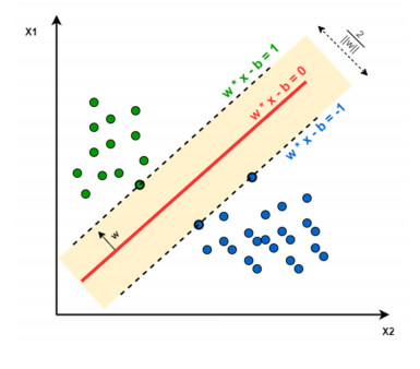
Support vector machines (SVMs) belong to a class of generalized linear classifiers used for binary data classification in supervised learning (Figure 1). The decision boundary is defined as the optimal hyperplane that best separates the training samples. The primary objective of SVM is to find a hyperplane that maximizes the margin between different classes, ultimately transforming the problem into a convex quadratic programming task. Consider a simple two-dimensional space: if a linear function can accurately classify the data points, we say that the data are linearly separable. This linear function is commonly referred to as the classification hyperplane. In the case of linearly separable SVMs, the data samples can be correctly separated by a straight line, maximizing noise immunity and enhancing predictive performance.
The form in which a hyperplane can completely segment the sample data can be computed using a linear support vector machine. Given the input data and learning objectives, the optimal hyperplane can be described by the following linear equation:
| WTx+b=0 | (1) |
where W is the average vector determining the direction of the hyperplane and b is the displacement, which determines the distance of the hyperplane from the origin. Assuming that the hyperplane can classify the training samples correctly, for the training samples (xi, yi), the following equation is satisfied:
| yi(WTxi+b)≥±1 | (2) |
The formula is known as the maximum interval hypothesis. yi= +1 indicates a positive sample and yi= −1 indicates a negative sample. The sample points that satisfy the following formula are called support vectors.
| yi(WTxi+b)=1 | (3) |
The interval M is then equal to the projection of the difference of the dissimilar support vectors in the W direction, which can be derived by:
| M=(→x+−→x−)→WT||W||=1−b+1+b||W||=2||W|| | (4) |
The principle of SVM makes the interval maximized:
| min12||W||2s.t. yi(WTxi+b)≥±1 | (5) |
This is a convex quadratic programming problem that needs to be simplified by adding Lagrange multipliers αi≥0 to each constraint of the equation. Solving for its pairwise variations, the original problem is transformed into the following problem:
| max{a}∑mi=1ai−12∑mi=1∑mj=1aiajyiyjxixjs.t. m∑i=1aiyi=0,αi≥0,i=1,2,3,…,m | (6) |
The solutions to the SVM model are recovered by the following form after solving for α, W, and b:
| f(x)=WTx+b=∑mi=1aiyixTix+b | (7) |
For nonlinear problems, linearly differentiable SVM is not a practical solution, and a nonlinear SVM model should be used for better classification. The same is true for transforming the data from low-dimensional to high-dimensional space so that the sample data in the high-dimensional space is linearly separable. Let ϕ(x)denote the feature vector after mapping x, and the division of the hyperplane corresponding to the model can be expressed as:
| f(x)=WTϕ(x)+b=0 | (8) |
Thus, one arrives at a minimizing function:
| min{w,b}12||W||2s.t. yi(WT∅(xi)+b)≥1(i=1,2,…,m) | (9) |
Its dyadic problem is:
| max{α}∑mi=1ai−12∑mi=1∑mj=1aiajyiyjϕ(xi)Tϕ(xj)s.t. m∑i=1aiyi=0,αi≥0,i=1,2,3,…,m | (10) |
The solution is formulated as:
| f(x)=WTϕ(x)+b=∑mj=1aiyiϕ(xi)Tϕ(xj)+b=∑mj=1aiyiκ(xi,xj)+b | (11) |
where the function κ(xi,xj) is the kernel function.
The most widely used kernel functions belong to four main types, having the most stable performance: the linear kernel function, polynomial kernel function, Gaussian kernel function, and sigmoid kernel function. In this paper, the linear kernel function is chosen based on the following advantages. The linear classification function is relatively simple and is suitable for linearly differentiable cases. It is faster to train with linear functional kernels, which avoids high computational complexity. Its decision boundaries can be explicitly interpreted and easily understood and explained.
SVR is a robust and commonly used regression algorithm that maximizes the spacing between the sample data points and the hyperplane as much as possible by finding a hyperplane in the feature space while controlling the error within a specific range. In SVR, we can define the regression problem in the following form:
| yi=f(xi)+ϵi | (12) |
where yi is the actual target value of the sample, xi is the input feature, f(xi) is the predicted output of the SVR regression function, and ϵi is the prediction error.
The goal of SVR is to find an optimal hyperplane such that the data points closest to the actual sample values on that hyperplane are called support vectors and such that there are as few sample points in the interval as possible. In this way, the model can better adapt to the characteristics of the data and, at the same time, have a high generalization ability.
In Figure 2, an SVR hyperplane and support vectors are depicted in a 2D feature space schematically.

The SVR hyperplane is a straight line whose position and slope are determined by the model parameters. Positive and negative intervals are two straight lines parallel to the hyperplane, and the model's interval parameter determines their distance from the hyperplane. The support vectors are the closest data points to the hyperplane, and they play a vital role in the training and prediction of the model.
Choosing different kernel functions can give SVR different nonlinear capabilities. Commonly used kernel functions are the polynomial kernel function, Gaussian kernel function, and sigmoid kernel function. These kernel functions can map the sample data into a high-dimensional feature space for nonlinear regression.
Predicting a stock's upward or downward trend is a two-class classification problem. The logistic regression model can provide both class probability estimation and improve prediction accuracy. By combining the analysis of emotions on the development of the financial market, some critical technical indicators are selected as predictive vectors. The upward and downward trend of the stock is treated as a binary response variable Y. A logistic regression model using these technical indicators is established to learn and predict the stock trend. Logistic regression assumes that the data obeys this distribution and then uses excellent likelihood estimation to estimate parameters. Logistic regression is a classical machine learning algorithm widely used in many fields. It can be used not only for binary classification problems but can also be extended for multiclassification problems with some tricks. The basic idea of logistic regression is to classify the output of a linear regression model by mapping it to a probability value and using a threshold. The basic formula for the logic function is as follows:
| h(x)=11+e−z | (13) |
where h(x) denotes the probability that sample x belongs to the positive class, and z is the output of the linear regression model, which can be expressed as:
| z=θ0+θ1x1+θ2x2+⋯+θnxn | (14) |
where θ0,θ1,…,θn are the parameters of the model, and x1,x2,…,xn are input features.
The training process for a logistic regression model involves determining the values of the parameters through maximum likelihood estimation. The goal of maximum likelihood estimation is to maximize the probability of the model's predicted outcome given the training data. Specifically, for the binary classification problem, we can define the likelihood function as:
| L(θ)=∏mi=1h(x(i))y(i)(1−h(x(i)))1−y(i) | (15) |
where m is the number of training samples, x(i) is the feature of the i sample, and y(i) is the label of the i sample.
In practice, it is common to take the logarithm of the likelihood function to get the log-likelihood function for ease of calculation:
| logL(θ)=∑mi=1[y(i)log(h(x(i)))+(1−y(i))log(1−h(x(i)))] | (16) |
The log-likelihood function can be used as a loss function to update the model's parameters through optimization algorithms such as gradient descent θ, which makes the model's predictions as close as possible to the actual labels.
The logistic regression model is a simple and efficient classification algorithm with the advantages of being interpretable, handling linearly separable and indivisible problems, and estimating probabilities. However, the logistic regression model requires high feature engineering and is prone to be affected by outliers. Therefore, when applying the logistic regression model, it is necessary to weigh the specific problems' characteristics and perform appropriate feature engineering and model tuning.
Random forest is an integrated learning method that makes collective decisions by constructing multiple decision tree models. It performs well in classification and regression tasks and has high robustness and predictive performance. The random forest model consists of multiple decision trees, each trained based on randomly selected training samples and features. In constructing each decision tree, random forest uses bootstrap sampling, i.e., samples equal to the size of the original training set are randomly sampled from the original training set with put back as training data. In addition, for each node split of the decision tree, random forest randomly selects a portion of the features to be evaluated instead of considering all the features. Through this integrated learning approach, random forest can enhance the robustness and accuracy of the model by voting or averaging the prediction results among the decision trees. It can effectively solve the overfitting problem and has good generalization ability.
The decision tree is an algorithm based on tree structure, often applied to handle classification and regression problems. Usually, a complete decision tree has three central nodes: the root node, the internal node, and the leaf node. The root node is unique while the internal node and the leaf node can be many. The root node and the internal nodes are the nodes where the selection division is performed, and the test data samples obtained are their respective nodes based on the determined selection division basis. This continuous selection process stops when the final predicted attribute value can be obtained after the division. The specific decision tree partitioning model is shown in Figures 3 and 4.


The essence of the decision tree algorithm is to obtain the division criteria for each node; when the specification of the division criteria for a particular problem criterion is obtained, it can be trained using the training data and predicted on the prediction data. Of course, selecting such division criteria is the process of finding the optimal decision tree; we expect to obtain division criteria with a good performance not only in the training set but also in the prediction set. There cannot be an overfitting state that works well on the training set while the prediction set division fails. Attribute determination, spanning trees, and pruning are critical to this problem. Attribute determination is the most important. Generally, purity is used to measure the distribution trend of the nodes; the higher the purity, the better. Generally speaking, there are three standard evaluation metrics to measure purity: information gain, gain rate, and the Gini coefficient, explicitly calculated as follows: If the sample set is defined as D, the share owned by the kth data is pk, k=1,2,…,|y|, remembering that each of the attributes of the dataset, α, has V elements {a1,a2,…,aV}.
(1) Information gain
Defining the information entropy of D:
| Ent(D)=−∑|y|k=1pklog2pk | (17) |
Then, the information gain obtained from the delineation of the attribute α to the sample set D is defined as:
| Gain(D,a)=Ent(D)−∑VV=1|DV||D|Ent(DV) | (18) |
(2) Gain ratio
The information gain ratio obtained by dividing the sample set D by the attribute a is defined as:
| Gain_ratio(D,a)=Gain(D,a)IV(a) | (19) |
where IV(a)=−∑VV=1|DV||D|log2|DV||D| represents the sample set D entropy concerning the values of the attribute α.
(3) Gini index
The Gini value is first calculated as:
| Gini(D)=∑|y|k=1∑k′≠kpkpk′=1−∑|y|k=1p2k | (20) |
Then, the Gini coefficient for an attribute is defined as:
| Gini_index(D,a)=∑VV=1|DV||D|Gini(DV) | (21) |
The decision tree model prioritizes optimal values within its components. Based on the three mentioned metrics, it compares different decision trees and selects the best-performing metrics to construct the final decision tree. In contrast, during pruning, the focus shifts to overall value optimization. The goal is to prevent excessive alignment with the training set, thereby achieving better results on the test set and enhancing decision tree prediction accuracy. This modeling method involves constant downward splitting of branches, making it easier to comprehend. While its computational complexity remains relatively low, extreme outliers can impact accuracy. Decision trees have limitations in handling imperfect data, leading scholars to favor ensemble learning—a blend of multiple algorithms—to enhance prediction accuracy. Random forest serves as an improvement over the decision tree for addressing overfitting and enhancing prediction accuracy.

The random forest classification algorithm integrates decision trees, offering high classification accuracy and robustness. Initially, it constructs multiple decision trees by randomly sampling from the original dataset (with replacement). To enhance classifier diversity, each tree randomly selects a feature subset during node splitting. Classification results from all trees are combined via voting, yielding the final prediction. Random forests handle samples and features with randomness, resulting in better overfitting resistance and generalization. Widely used in medical diagnosis, image processing, and financial risk analysis, this method excels. Similarly, random forest regression addresses regression problems. It constructs multiple decision trees using self-sampling, with each tree randomly selecting feature subsets for segmentation. The final regression value is an average of all tree predictions. This integrated approach enhances regression model accuracy, robustness, and feature importance assessment. Random forest regression finds applications in financial risk prediction, sales volume forecasting, and house price estimation.
The daily index data of the CSI 300 index from January 1, 2006 to June 30, 2023 are selected, including the lagged 20-day closing price (Close), volume, short-term rolling moving average of closing price (MA10), long-term rolling moving average of closing price (MA30), relative strength indicator (RSI), amplitude, and mean average of closing price (MA30). Amplitude, mean cross characteristics (MA10_cross_MA30), overbought and oversold indicators (CCI), up and down (Change), stock turnover, overnight yield, and other indices are the most critical indicators of volume and investor sentiment. The data used were available at the WIND database at the library of the first author's affiliated university when the current study was being carried out. Important features such as daily closing price (Close) with a lag of 20 days, volume, relative strength indicator (RSI), amplitude, SMA crossover feature (MA10_cross_MA30), overbought and oversold category indicator (CCI), change, stock turnover, overnight yield, etc. were used as the main features extracted for stock price trend prediction.
We used the Jarque-Bera (JB) statistic to evaluate the distribution of each factor, revealing significant deviations from normality. For example, the closing and opening prices have JB statistics of 24.98 and 24.70, with p-values well below 0.05, indicating non-normality despite near-normal skewness and kurtosis. The trade volume, with high skewness, kurtosis, and a long tail, has a JB statistic of 21424.71 and a p-value of 0, highlighting a strong deviation from normality. While the JB test is sensitive to large sample sizes, making even minor deviations appear significant, the results suggest non-normality in our data. We will explore whether machine learning models can handle these non-normal distributions and assess their performance in this context. Descriptive statistics are summarized in Table 1.
| Factors | Std | Min | 50% | Max | Skewness | Kurtosis | JB Statistic | P-value |
| Close | 980.75 | 1004.34 | 3354.89 | 5877.20 | 0.05 | −0.36 | 24.98 | 3.77E-06 |
| Open | 982.25 | 1004.75 | 3349.70 | 5922.07 | 0.06 | −0.36 | 24.70 | 4.34E-06 |
| Volume | 7.85E+09 | 1.13E+09 | 8.66E+09 | 6.86E+10 | 2.59 | 9.76 | 21424.71 | 0 |
| close − 1d | 981.99 | 1004.34 | 3354.17 | 5877.20 | 0.05 | −0.36 | 24.59 | 4.57E-06 |
| close − 20d | 993.86 | 983.62 | 3342.63 | 5877.20 | 0.03 | −0.34 | 21.39 | 2.27E-05 |
| MA5 | 981.24 | 1011.47 | 3351.84 | 5804.01 | 0.05 | −0.36 | 24.71 | 4.31E-06 |
| MA10 | 981.27 | 1019.39 | 3343.36 | 5726.47 | 0.04 | −0.37 | 24.64 | 4.45E-06 |
| MA30 | 981.09 | 1006.90 | 3343.30 | 5572.04 | 0.01 | −0.37 | 24.72 | 4.3E-06 |
| RSI | 13.46 | 17.15 | 51.62 | 93.80 | 0.24 | −0.41 | 70.70 | 4.44E-16 |
| BB_upper | 1005.16 | 1022.24 | 3430.27 | 5978.91 | 0.06 | −0.33 | 22.35 | 1.4E-05 |
| BB_middle | 981.24 | 1011.47 | 3351.84 | 5804.01 | 0.05 | −0.36 | 24.71 | 4.31E-06 |
| BB_lower | 961.08 | 990.72 | 3289.47 | 5704.19 | 0.04 | −0.38 | 27.38 | 1.14E-06 |
| Momentum | 188.43 | −1217.09 | 16.07 | 743.24 | −0.68 | 4.26 | 3495.58 | 0 |
| MA14 | 981.28 | 1025.27 | 3338.91 | 5674.73 | 0.03 | −0.37 | 24.61 | 4.52E-06 |
| MA10_cross_MA30 | 1.00 | −1.00 | 1.00 | 1.00 | −0.19 | −1.97 | 703.37 | 1.8E-153 |
| CCI5 | 95.28 | −166.67 | 18.52 | 166.67 | −0.13 | −1.29 | 304.90 | 6.18E-67 |
| CCI10 | 105.55 | −308.83 | 19.32 | 271.79 | −0.16 | −0.88 | 154.67 | 2.59E-34 |
| CCI14 | 109.30 | −382.42 | 20.13 | 331.86 | −0.20 | −0.73 | 121.83 | 3.51E-27 |
| Inter_return | 0.75 | −9.09 | −0.03 | 8.96 | 0.18 | 31.30 | 171825.90 | 0 |
| Turn_growth | 0.24 | −2.41 | −0.01 | 1.93 | 0.17 | 13.32 | 31139.85 | 0 |
 DownLoad:
CSV
DownLoad:
CSV
As different indicators characterize different information and have different value spans, it is necessary to preprocess the data to increase the smoothness of the model training. In normalizing the data, the mean ˉx and standard deviation S of the features need to be calculated, and the normalization equation is as follows:
| x′=x−ˉxS |
The initial data is X={x1,x2,…,xn}, with xmin as the minimum and xmax as the maximum, and the difference between the maximum and minimum is utilized for the normalization process to make the initial data at a level that does not bring about excessive quantitative differences, and which can lead to more accurate model results.
| xnorm=x−xminxmax−xmin |
When dealing with a substantial amount of data, features and normalizations become necessary during data processing. If there is abundant input data and only a small amount of missing data—particularly when the overall dataset proportion is low—the impact of those missing values on the entire dataset is negligible. In such cases, opting to delete the missing data directly helps maintain data integrity. However, when there is a more significant amount of missing data that cannot be ignored outright, an alternative approach is to use the mean value to fill in the gaps. This strategy ensures data integrity while accounting for missing information. In this study, normalization is employed to standardize the data. The normalized data are as follows (Table 2):
| Open | Volume | MA5 | RSI | BB_upper | Momentum | CCI10 | Inter_return | Turn_growth |
| −2.35984 | −1.09093 | −2.36812 | 1.328269 | −2.3749 | 0.054993 | 1.104699 | 0.168912 | −0.03407 |
| −2.34561 | −1.05021 | −2.36278 | 1.243441 | −2.37834 | 0.050374 | 1.076513 | 0.917889 | 0.983727 |
| −2.35502 | −1.09504 | −2.35989 | 1.366777 | −2.37394 | 0.041085 | 0.627325 | −0.05133 | −1.13981 |
| −2.34988 | −1.09412 | −2.35607 | 1.451149 | −2.37095 | 0.043633 | 0.979435 | −0.06568 | 0.019875 |
| −2.3457 | −1.02466 | −2.35662 | 0.534536 | −2.36969 | 0.06269 | 0.158751 | −0.00337 | 1.745378 |
DownLoad:
CSV
For regression algorithms, we evaluate it by the size of the difference between its predicted results and our actual results. In the regression algorithm, the four most commonly used evaluation indexes are the mean square error (MSE), root mean square error (RMSE), mean absolute error (MAE), and resolvable coefficient (R-Square).
In binary classification, we evaluate the performance of classification methods based on their actual and predicted categories, by breaking down the four possible outcomes as follows. True positive (TP): These are instances where the model correctly predicts the positive class (e.g., correctly identifying a disease in a medical test). False positive (FP): These occur when the model predicts the positive class incorrectly (e.g., a false alarm in a spam filter). True negative (TN): These are instances where the model correctly predicts the negative class (e.g., correctly identifying a non-disease case in a medical test). False negative (FN): These occur when the model predicts the negative class incorrectly (e.g., failing to detect a disease in a medical test). Insights into the overall performance of the classification model can be gained by various manipulations of these four indicators, including the accuracy rate and recall rate.
The prediction interval is the test set time for the stock index movement data, i.e., January 2021 to June 2023. The following figure shows the confusion matrix for the three machine learning classification models.


According to Table 3 and Table 4, the prediction effect of the five machine learning model algorithms varies. The regression model performs with a decision coefficient of 0.9793, but its MAE and RMSE indicators are not as favorable. In contrast, the classification machine learning model shows better performance, with very good MAE and RMSE indices, and an accuracy rate of about 50%. Specifically, comparing these models reveals that the classification prediction generally scores better, with lower MSE and MAE values, and a more significant decision coefficient. We believe that in the CSI 300 index prediction in the last 17 years, the regression model has a particular advantage. However, as to whether different machine learning models have similar effects when applied to the real market, we conduct a comprehensive backtesting analysis and comparison.
| Model | Metric | Negative | Positive |
| LR | True Positives (TP) | - | 187 |
| False Negatives (FN) | - | 101 | |
| False Positives (FP) | 217 | - | |
| True Negatives (TN) | 94 | - | |
| SVM | True Positives (TP) | - | 115 |
| False Negatives (FN) | - | 173 | |
| False Positives (FP) | 117 | - | |
| True Negatives (TN) | 194 | - | |
| RF | True Positives (TP) | - | 186 |
| False Negatives (FN) | - | 102 | |
| False Positives (FP) | 191 | - | |
| True Negatives (TN) | 120 | - |
DownLoad:
CSV
| LR | SVM | RF Classification | SVR | RF Regression | |
| Accuracy | 0.472461 | 0.512150 | 0.516955 | - | - |
| Recall | 0.475778 | 0.511550 | 0.515843 | - | - |
| F1 Score | 0.456001 | 0.507290 | 0.504840 | - | - |
| MAE | 1.061769 | 0.968281 | 0.978297 | 6073.132 | 10312.05 |
| MSE | 2.123539 | 1.936560 | 1.956594 | 57.68090 | 78.78598 |
| RMSE | 1.457236 | 1.391604 | 1.398783 | 77.930302 | 101.5482 |
| R2 | −1.126674 | −0.939420 | −0.959483 | 0.979388 | 0.965001 |
DownLoad:
CSV
Specifically, this paper selects MSE, RMSE, MAE, and R² as the prediction evaluation metrics. After model training and data prediction, we assessed the effectiveness of the models from the perspective of predicting the different evaluation metrics. The evaluation results found that the classification models performed better in predicting the CSI 300 index in the last two years used in this paper, in which the support vector machine classification model showed the best performance, while the other logistic regression classification model presented the worst performance. This chapter provides a preliminary assessment of the fitting results of different machine learning models; whether these models still have the same results in real scenarios will be further verified by constructing quantitative strategies for backtesting in the next section.
Generally speaking, there are two common ways to apply machine learning models to quantitative investment. One is the quantitative timing strategy. Quantitative timing is to analyze different macro and micro indicators through quantitative methods to find the main factors affecting the fluctuation of stock prices, achieve a more accurate prediction of the subsequent market trend, choose the appropriate trading signals, and buy and sell to obtain strategic returns. The other is the quantitative stock selection strategy. Quantitative stock selection uses quantitative techniques to select a portfolio of stocks, expecting the selected portfolio to have a higher rate of excess return, generally utilizing fundamentals and technical indicators for stock selection. In this chapter, we choose the former for strategy construction and use the machine learning model constructed in the previous chapter to realize strategy returns by predicting the general market trend and selecting the trading time. Our construction of the timing strategy is as follows:
(1) Tool selection: The strategy writing tools and data sources include Python, Tushare, and Wind financial terminal trading data. The strategy can be edited to generate backtesting charts directly, which is convenient for extracting data for the paper and easy for readers to understand. This article uses Numpy, Pandas, and Talib packages in the Python programming language for data processing and factor construction; Matplotlib and Seaborn packages for drawing; and Pytorch, Keras, Sklrean, and Tensorflow packages to build machine learning models.
(2) Backtesting time: January 1, 2021–June 30, 2023. This interval spans two and a half years and is close to the time of writing this paper. The period includes a certain degree of volatility in the CSI 300 index trend, including both downward and upward intervals, making it suitable for backtesting.
(3) Benchmark return: CSI 300 Index for the same period.
(4) Positioning frequency: daily.
(5) Timing signal: Utilizing a machine learning timing strategy, bilateral trading is conducted. Various machine learning algorithms predict the stock price situation for the next day, serving as the foundation for generating both open long and open short signals.
The specific rules for classification and regression strategies are as follows: Based on the closing price of the day, use the different machine learning algorithms to predict whether the next day's movement will be up by 1 or down by −1, to open long or short positions, respectively. Calculate the stock price for the next day using different machine learning algorithms. Model for the regression methodology predicted for the stock price, while ensuring model accuracy. Open long conditions if the second-day closing price is greater than the second-day opening price plus 0.1 times the 20-day rolling standard deviation, and vice versa for short conditions.
In order to compare the performance of different quantitative trading strategies, this paper selects the following indicators to assess the strategy indicators.
| TotalReturns=Pend−PstartPstart∗100% |
| TotalAnnualizedReturns=Rp=((1+P)250n−1)∗100% |
| ExcessReturns=StrategyReturns−BenchmarkReturns |
| MaxDrawdown=Max(Px−Py)Px |
| SharpeRatio=Rp−Rfσp |
where Pend= Total assets at the end of the strategy; Pstrart=Total assets at strategy start; P = Strategy return; n = Number of days of strategy execution; Px, Py = Total value of stocks and cash on a given day of the strategy, y>x; Rp = Strategy annualized return; Rf = Risk-free rate (default 0.02); σp = Strategy return volatility.
A comparison of the overall return movements over the backtesting interval after executing the live backtesting results for different machine learning training models is shown in Figure 11 and Figure 12. The results of the above five machine learning model backtesting evaluation metrics and benchmarking indices are presented in Table 5.


| CSI300 | LR | SVM | RF classification | SVR | RF regression | |
| Strategy returns | −30.45% | −7.60% | 30.27% | 8.68% | 3.15% | 25.03% |
| Total annualized returns | −14.09% | −3.25% | 11.69% | 3.54% | 1.31% | 9.79% |
| Excess returns | − | 22.78% | 60.52% | 39.01% | 32.21% | 53.75% |
| Max drawdown | 39.59% | 27.30% | 16.10% | 23.70% | 16.94% | 22.35% |
| Sharpe ratio | - | −0.28 | 0.42 | 0.08 | −0.14 | 0.32 |
DownLoad:
CSV
The SVM and RF regression strategies perform better regarding strategy returns, annualized returns, and excess returns. They have positive returns and exceed the benchmark returns. However, the RF regression strategy has a higher maximum retracement of 22.35%. Regarding risk tolerance, the Sharpe ratio is positive, indicating that the strategy performs better in return relative to the risk taken. The SVM classification strategies have relatively low maximum retraction and positive Sharpe ratios, indicating that they perform better in return than the risk taken.
SVM and RF regression strategies have exceptionally high returns. In particular, the SVM strategy has annualized and excess returns of 11.69% and 60.52%, respectively. However, the maximum retracements of the RF regression strategy are relatively larger than SVM, indicating that its performance is relatively unstable when the market falls. However, it is much smaller than the maximum decline of the index in the same period.
Considering the factors of return, risk, and stability, investors should choose the appropriate strategy according to their investment objectives and risk tolerance. SVM strategy has better overall performance. In contrast, random forest regression strategies have excess returns but may have more significant retracements. When selecting a strategy, investors should consider the indicators and compare them with other strategies or markets to fully assess their performance.
In conclusion, this study analyzes the CSI 300 index using various strategies and evaluates their performance. The results provide a valuable reference for investors when making investment decisions. However, it should be noted that changes and uncertainties in the market may impact the performance of the strategies, so investors should be cautious in evaluating and adjusting their strategies to the changes in the market in practice. In addition, our selected backtesting intervals belong to the downward range with oscillating market intervals. There is also a relationship between the selection of backtesting intervals and the model simulation.
The following figure used more common regression and neural network models on the market to add feature factor strategies for comparison, including least squares OLS regression, LASSO regression, ridge regression, and long- and short-term memory recurrent neural network methods (LSTM) to compare with the SVR strategy. The strategy results are shown below (Figure 13).

As seen from the above chart, as of June 30, 2023, except for the LASSO regression, the returns of other models have remained at a low level (Table 6). However, all have excess returns, which can be roughly inferred as due to the effectiveness of the factor selection of the inputs. The return on long short-term memory network (LSTM) is relatively low, and the LSTM model is susceptible to the selection and representation of input features. Suppose the selected features do not have sufficient information or have a weak relationship with the target variable. In that case, the model may not predict accurately, resulting in lower returns. Regression performs well in the characteristic factor strategy, especially the ordinary least squares (OLS) regression, ridge regression, and LASSO regression. However, each model has its strengths and limitations, and choosing the most suitable model for a particular problem and dataset is essential.
| LASSO | OLS | Ridge | LSTM | |
| Strategy returns | −5.29% | 4.84% | 0.88% | −8.17% |
| Total annualized returns | −2.25% | 2.00% | 0.37% | −3.50% |
| Excess returns | 23.90% | 33.88% | 29.98% | 21.07% |
| Max drawdown | 16.58% | 24.78% | 21.85% | 22.25% |
| Sharpe ratio | −0.0001 | −0.23 | −0.09 | −0.30 |
DownLoad:
CSV
In this paper, we leverage the timing of trading, using the CSI 300 index as the benchmark, to determine the trading signals, and construct the quantitative strategy. We choose strategy return, strategy annualized return, excess return, maximum retracement rate, and Sharpe ratio as the evaluation indexes of the strategy. In the end, several models have obtained returns exceeding the accurate market benchmark. The categorical models in this paper have average performance and similar evaluation metrics regarding risk and return. However, the regression models are the best performers, especially the SVM model, with an excess return of 60.52%. In the end, the regression method, which is used more often in the market literature, is added to the strategy and also shows a better performance in terms of returns, which also indicates that the selection of the characteristic factors is more effective.
This study explores stock price movement patterns, using various algorithmic machine learning models. China's stock exchange market is relatively nascent compared to Europe and the United States. Stock price dynamics are influenced not only by the business performance of leading companies but also by domestic and peripheral market trends, news, public opinion, and overall market sentiment. Traditional research methods often fall short in this intricate system. With a plethora of machine learning algorithms available, prediction accuracy varies based on parameters and market contexts. By analyzing different algorithms and testing with real data, the study provides innovative approaches for stock price prediction particularly in China's market. Furthermore, the long-standing assumption of "rational actors" in financial research has been challenged. Investor emotions and irrational behaviors have been recognized as critical factors that significantly impact financial markets. These irrational and sentiment factors have been successfully incorporated into the machine learning models of the current study. The success of the models in this study aligns with findings in the literature, supporting their role in financial forecasting (Chen and Guestrin, 2016). Machine learning models, including LSTM networks, have been widely recognized as effective tools for handling time series data, consistent with other research results (Behera et al., 2020). However, while previous studies have extensively explored the application of traditional machine learning models (Tsay, 2013), this study offers a more detailed machine learning strategy method. The practical application of parameter settings and model tuning may differ across markets, especially when compared to findings from more mature markets like those in the United States or Europe.
The presence of significant deviations from normality in the data, as indicated by the JB test results, suggests that the models might not fully account for non-normal distribution characteristics. This non-normality could affect prediction accuracy, and while adjustments can be made, they may not completely resolve the underlying issues. Additionally, the prediction accuracy could potentially be further enhanced by exploring other algorithms such as XGBoost. It is also important to recognize that economic conditions, unexpected events, and capital flows significantly impact stock prices. To improve predictions, incorporating a broader range of factors, such as macroeconomic policy outlooks, meso-level industry analyses, and micro-level company-specific news or statements, could provide a more comprehensive understanding and potentially enhance model performance. In the current study, we use default values for most parameters of various machine learning models, where the practicality varies in the different markets. There are various methods including window partitioning to address the autocorrelations, which are commonly observed in time series data (Akhtar et al., 2022). However, with daily frequency data, such methods could lead to small training sets and insufficient model training. Akhtar et al. (2022) and Behera et al. (2020) found traditional machine learning models mostly effective for temporal data prediction. The current study also employs LSTM neural networks, which are well-suited for time series data. The use of machine learning for time series prediction remains a promising area for future research.
This research focuses on constructing the optimal machine learning algorithms for price prediction and profit-making in the stock market by employing the representative CSI 300 index as the dataset for the proposed models. The training dataset spans from the beginning of 2006 to the end of 2020, while the prediction dataset covers the period from the start of 2021 to June 2023. Five machine learning models are utilized for prediction: logistic regression, support vector machine, support vector regression, random forest classification, and random forest regression. For regression-based predictions related to stock price indices, the following evaluation metrics are selected: MSE, MAE, RMSE, and R². By comparing the effectiveness of these models using the specified evaluation criteria, it is observed that the regression models outperform other approaches in prediction accuracy.
To assess the impact of various machine learning models, we construct and implement quantitative trading strategies suited to the real-world market. The results reveal that the predictive efficacy of the constructed machine learning models surpasses the benchmark return. Notably, the support vector regression model stands out, achieving a remarkable return rate exceeding 60% in actual market predictions. Additionally, the backtesting returns for the remaining models also outperform the benchmark, underscoring the importance of relevant technical indicators—such as investor sentiment—in feature selection. Furthermore, the effectiveness of this forecasting approach hinges on both model selection and the choice of the backtesting interval. The findings provide valuable insights for leveraging machine learning techniques in predicting financial time series data and constructing quantitative strategies.
In our study, we employed the CSI 300 index as the benchmark to develop a timing strategy for backtesting. Alternatively, we could utilize either the CSI 300 or the entire A-share market as the stock pool for constructing a backtesting strategy. In this context, various machine learning methods exhibit differing performance. Notably, incorporating the investor sentiment characteristic factor has demonstrated improved predictive efficacy when comparing different model algorithms. For future research, fine-tuning model algorithm parameters and reconfiguring the model architecture could enhance prediction accuracy.
The authors' contributions to this study are equal.
The authors declare they have not used Artificial Intelligence (AI) tools in the creation of this work.
All authors declare no conflicts of interest in this work.
| [1] |
Akhtar MM, Zamani AS, Khan S, et al. (2022) Stock market prediction based on statistical data using machine learning algorithms. J King Saud University-Sci 34: 101940. https://doi.org/10.1016/j.jksus.2022.101940 doi: 10.1016/j.jksus.2022.101940

|
| [2] |
Baker M, Stein JC (2004) Market liquidity as a sentiment indicator. J Financ Mark 7: 271–299. https://doi.org/10.1016/j.finmar.2003.11.005 doi: 10.1016/j.finmar.2003.11.005
|
| [3] |
Balcilar M, Bonato M, Demirer R, et al. (2017) The effect of investor sentiment on gold market return dynamics: Evidence from a nonparametric causality-in-quantiles approach. Resour Policy 51: 77–84. https://doi.org/10.1016/j.resourpol.2016.11.009 doi: 10.1016/j.resourpol.2016.11.009
|
| [4] |
Barberis N, Shleifer A, Vishny R (1998) A model of investor sentiment. J Financ Econ 49: 307–343.. https://doi.org/10.1016/S0304-405X(98)00027-0 doi: 10.1016/S0304-405X(98)00027-0
|
| [5] |
Behera RK, Das S, Rath SK, et al. (2020) Comparative Study of Real Time Machine Learning Models for Stock Prediction through Streaming Data. J Univers Comput Sci 26: 1128–1147. https://doi.org/10.3897/jucs.2020.059 doi: 10.3897/jucs.2020.059
|
| [6] |
Cao X, Xing L, Majd E, et al. (2022) A systematic evaluation of supervised machine learning algorithms for cell phenotype classification using single-cell RNA sequencing data. Front Genet 13: 836798. https://doi.org/10.3389/fgene.2022.836798 doi: 10.3389/fgene.2022.836798
|
| [7] |
Chau F, Deesomsak R, Koutmos D (2016) Does investor sentiment really matter? Int Rev Financ Anal 48: 221–232. https://doi.org/10.1016/j.irfa.2016.10.003 doi: 10.1016/j.irfa.2016.10.003
|
| [8] | Chen T, Guestrin C (2016) Xgboost: A scalable tree boosting systemProceedings of the 22nd acm sigkdd international conference on knowledge discovery and data mining. |
| [9] |
Da Z, Engelberg J, Gao P (2015) The sum of all FEARS investor sentiment and asset prices. Rev Financ Stud 28: 1–32. https://doi.org/10.1093/rfs/hhu072 doi: 10.1093/rfs/hhu072
|
| [10] |
De Long JB, Shleifer A, Summers LH, et al. (1990) Noise trader risk in financial markets. J Polit Econ 98: 703–738. https://doi.org/10.1086/261703 doi: 10.1086/261703
|
| [11] |
Dong Y, Zhou S, Xing L, et al. (2022) Deep learning methods may not outperform other machine learning methods on analyzing genomic studies. Front Genet 13: 992070. https://doi.org/10.3389/fgene.2022.992070 doi: 10.3389/fgene.2022.992070
|
| [12] |
Frugier A (2016) Returns, volatility and investor sentiment: Evidence from European stock markets. Res Int Bus Financ 38: 45–55. https://doi.org/10.1016/j.ribaf.2016.03.007 doi: 10.1016/j.ribaf.2016.03.007
|
| [13] |
Green J, Hand JR, Zhang XF (2013) The supraview of return predictive signals. Rev Account Stud 18: 692–730. https://doi.org/10.1007/s11142-013-9231-1 doi: 10.1007/s11142-013-9231-1
|
| [14] | Gu Y, Xu S (2022) The Impact of Investor Sentiment on The Stock Market——Based on The Research of China's A-Share Market, 2022 2nd International Conference on Management Science and Industrial Economy Development (MSIED 2022). https://doi.org/10.23977/msied2022.022 |
| [15] |
Harvey CR, Liu Y, Zhu H (2016) … and the cross-section of expected returns.Rev Financ Stud 29: 5–68. https://doi.org/10.1093/rfs/hhv059 doi: 10.1093/rfs/hhv059
|
| [16] |
He Z, He L, Wen F (2019) Risk compensation and market returns: The role of investor sentiment in the stock market. Emerg Mark Financ Trade 55: 704–718. https://doi.org/10.1080/1540496X.2018.1460724 doi: 10.1080/1540496X.2018.1460724
|
| [17] | Khaidem L, Saha S, Dey SR (2016) Predicting the direction of stock market prices using random forest. arXiv preprint arXiv: 1605.00003. https://doi.org/10.48550/arXiv.1605.00003 |
| [18] |
Khemchandani R, Chandra S (2009) Regularized least squares fuzzy support vector regression for financial time series forecasting. Expert Syst Appl 36: 132–138. https://doi.org/10.1016/j.eswa.2007.09.035 doi: 10.1016/j.eswa.2007.09.035
|
| [19] |
Kim Kj (2003) Financial time series forecasting using support vector machines. Neurocomputing 55: 307–319. https://doi.org/10.1016/S0925-2312(03)00372-2 doi: 10.1016/S0925-2312(03)00372-2
|
| [20] |
Lee CM, Shleifer A, Thaler RH (1991) Investor sentiment and the closed‐end fund puzzle. J Financ 46: 75–109. https://doi.org/10.1111/j.1540-6261.1991.tb03746.x doi: 10.1111/j.1540-6261.1991.tb03746.x
|
| [21] |
Li M, Esfahani F, Xing L, et al. (2023) Predicting the daily counts of COVID-19 infection using temporal convolutional networks. J Glob He 13. https://doi.org/10.7189/jogh.13.03029 doi: 10.7189/jogh.13.03029
|
| [22] |
Li X, Sun Y (2020) Stock intelligent investment strategy based on support vector machine parameter optimization algorithm. Neural Comput Appl 32: 1765–1775. https://doi.org/10.1007/s00521-019-04566-2 doi: 10.1007/s00521-019-04566-2
|
| [23] |
Lin CB, Chou RK, Wang GH (2018) Investor sentiment and price discovery: Evidence from the pricing dynamics between the futures and spot markets. J Bank Financ 90: 17–31. https://doi.org/10.1016/j.jbankfin.2018.02.014 doi: 10.1016/j.jbankfin.2018.02.014
|
| [24] |
Qiang Z, Shu-e Y (2009) Noise trading, investor sentiment volatility, and stock returns. Syst Eng-Theory Pract 29: 40–47. https://doi.org/10.1016/S1874-8651(10)60010-5 doi: 10.1016/S1874-8651(10)60010-5
|
| [25] | Tsay RS (2013) Multivariate time series analysis: with R and financial applications, John Wiley & Sons. |
| [26] | Webb A (2013) Fourier transform based investment styles on the Johannesburg Stock Exchange, University of Pretoria (South Africa). |
| [27] |
Wei C, Dan L (2019) Market fluctuation and agricultural insurance forecasting model based on machine learning algorithm of parameter optimization. J Intell Fuzzy Syst 37: 6217–6228. https://doi.org/10.3233/JIFS-179204 doi: 10.3233/JIFS-179204
|
| [28] |
Yang C, Li J (2013) Investor sentiment, information and asset pricing model. Econ Model 35: 436–442. https://doi.org/10.1016/j.econmod.2013.07.015 doi: 10.1016/j.econmod.2013.07.015
|
| [29] |
Yang C, Zhou L (2015) Investor trading behavior, investor sentiment and asset prices. North Am J Econ Financ 34: 42–62. https://doi.org/10.1016/j.najef.2015.08.003 doi: 10.1016/j.najef.2015.08.003
|
| [30] |
Zhang W, Gong X, Wang C, et al. (2021) Predicting stock market volatility based on textual sentiment: A nonlinear analysis. J Forecast 40: 1479–1500. https://doi.org/10.1002/for.2777 doi: 10.1002/for.2777
|
| [31] |
Zhang X, Huang Y, Xu K, et al. (2023) Novel modelling strategies for high-frequency stock trading data. Financ Innov 9: 39. https://doi.org/10.1186/s40854-022-00431-9 doi: 10.1186/s40854-022-00431-9
|
| [32] |
Zweig ME (1973) An investor expectations stock price predictive model using closed-end fund premiums. J Financ 28: 67–78. https://doi.org/10.2307/2978169 doi: 10.2307/2978169
|

Haoyu Wang, Dejun Xie. Optimal profit-making strategies in stock market with algorithmic trading[J]. Quantitative Finance and Economics, 2024, 8(3): 546-572. doi: 10.3934/QFE.2024021

| Factors | Std | Min | 50% | Max | Skewness | Kurtosis | JB Statistic | P-value |
| Close | 980.75 | 1004.34 | 3354.89 | 5877.20 | 0.05 | −0.36 | 24.98 | 3.77E-06 |
| Open | 982.25 | 1004.75 | 3349.70 | 5922.07 | 0.06 | −0.36 | 24.70 | 4.34E-06 |
| Volume | 7.85E+09 | 1.13E+09 | 8.66E+09 | 6.86E+10 | 2.59 | 9.76 | 21424.71 | 0 |
| close − 1d | 981.99 | 1004.34 | 3354.17 | 5877.20 | 0.05 | −0.36 | 24.59 | 4.57E-06 |
| close − 20d | 993.86 | 983.62 | 3342.63 | 5877.20 | 0.03 | −0.34 | 21.39 | 2.27E-05 |
| MA5 | 981.24 | 1011.47 | 3351.84 | 5804.01 | 0.05 | −0.36 | 24.71 | 4.31E-06 |
| MA10 | 981.27 | 1019.39 | 3343.36 | 5726.47 | 0.04 | −0.37 | 24.64 | 4.45E-06 |
| MA30 | 981.09 | 1006.90 | 3343.30 | 5572.04 | 0.01 | −0.37 | 24.72 | 4.3E-06 |
| RSI | 13.46 | 17.15 | 51.62 | 93.80 | 0.24 | −0.41 | 70.70 | 4.44E-16 |
| BB_upper | 1005.16 | 1022.24 | 3430.27 | 5978.91 | 0.06 | −0.33 | 22.35 | 1.4E-05 |
| BB_middle | 981.24 | 1011.47 | 3351.84 | 5804.01 | 0.05 | −0.36 | 24.71 | 4.31E-06 |
| BB_lower | 961.08 | 990.72 | 3289.47 | 5704.19 | 0.04 | −0.38 | 27.38 | 1.14E-06 |
| Momentum | 188.43 | −1217.09 | 16.07 | 743.24 | −0.68 | 4.26 | 3495.58 | 0 |
| MA14 | 981.28 | 1025.27 | 3338.91 | 5674.73 | 0.03 | −0.37 | 24.61 | 4.52E-06 |
| MA10_cross_MA30 | 1.00 | −1.00 | 1.00 | 1.00 | −0.19 | −1.97 | 703.37 | 1.8E-153 |
| CCI5 | 95.28 | −166.67 | 18.52 | 166.67 | −0.13 | −1.29 | 304.90 | 6.18E-67 |
| CCI10 | 105.55 | −308.83 | 19.32 | 271.79 | −0.16 | −0.88 | 154.67 | 2.59E-34 |
| CCI14 | 109.30 | −382.42 | 20.13 | 331.86 | −0.20 | −0.73 | 121.83 | 3.51E-27 |
| Inter_return | 0.75 | −9.09 | −0.03 | 8.96 | 0.18 | 31.30 | 171825.90 | 0 |
| Turn_growth | 0.24 | −2.41 | −0.01 | 1.93 | 0.17 | 13.32 | 31139.85 | 0 |
DownLoad:
CSV
| Open | Volume | MA5 | RSI | BB_upper | Momentum | CCI10 | Inter_return | Turn_growth |
| −2.35984 | −1.09093 | −2.36812 | 1.328269 | −2.3749 | 0.054993 | 1.104699 | 0.168912 | −0.03407 |
| −2.34561 | −1.05021 | −2.36278 | 1.243441 | −2.37834 | 0.050374 | 1.076513 | 0.917889 | 0.983727 |
| −2.35502 | −1.09504 | −2.35989 | 1.366777 | −2.37394 | 0.041085 | 0.627325 | −0.05133 | −1.13981 |
| −2.34988 | −1.09412 | −2.35607 | 1.451149 | −2.37095 | 0.043633 | 0.979435 | −0.06568 | 0.019875 |
| −2.3457 | −1.02466 | −2.35662 | 0.534536 | −2.36969 | 0.06269 | 0.158751 | −0.00337 | 1.745378 |
DownLoad:
CSV
| Model | Metric | Negative | Positive |
| LR | True Positives (TP) | - | 187 |
| False Negatives (FN) | - | 101 | |
| False Positives (FP) | 217 | - | |
| True Negatives (TN) | 94 | - | |
| SVM | True Positives (TP) | - | 115 |
| False Negatives (FN) | - | 173 | |
| False Positives (FP) | 117 | - | |
| True Negatives (TN) | 194 | - | |
| RF | True Positives (TP) | - | 186 |
| False Negatives (FN) | - | 102 | |
| False Positives (FP) | 191 | - | |
| True Negatives (TN) | 120 | - |
DownLoad:
CSV
| LR | SVM | RF Classification | SVR | RF Regression | |
| Accuracy | 0.472461 | 0.512150 | 0.516955 | - | - |
| Recall | 0.475778 | 0.511550 | 0.515843 | - | - |
| F1 Score | 0.456001 | 0.507290 | 0.504840 | - | - |
| MAE | 1.061769 | 0.968281 | 0.978297 | 6073.132 | 10312.05 |
| MSE | 2.123539 | 1.936560 | 1.956594 | 57.68090 | 78.78598 |
| RMSE | 1.457236 | 1.391604 | 1.398783 | 77.930302 | 101.5482 |
| R2 | −1.126674 | −0.939420 | −0.959483 | 0.979388 | 0.965001 |
DownLoad:
CSV
| CSI300 | LR | SVM | RF classification | SVR | RF regression | |
| Strategy returns | −30.45% | −7.60% | 30.27% | 8.68% | 3.15% | 25.03% |
| Total annualized returns | −14.09% | −3.25% | 11.69% | 3.54% | 1.31% | 9.79% |
| Excess returns | − | 22.78% | 60.52% | 39.01% | 32.21% | 53.75% |
| Max drawdown | 39.59% | 27.30% | 16.10% | 23.70% | 16.94% | 22.35% |
| Sharpe ratio | - | −0.28 | 0.42 | 0.08 | −0.14 | 0.32 |
DownLoad:
CSV
| LASSO | OLS | Ridge | LSTM | |
| Strategy returns | −5.29% | 4.84% | 0.88% | −8.17% |
| Total annualized returns | −2.25% | 2.00% | 0.37% | −3.50% |
| Excess returns | 23.90% | 33.88% | 29.98% | 21.07% |
| Max drawdown | 16.58% | 24.78% | 21.85% | 22.25% |
| Sharpe ratio | −0.0001 | −0.23 | −0.09 | −0.30 |
DownLoad:
CSV
| Factors | Std | Min | 50% | Max | Skewness | Kurtosis | JB Statistic | P-value |
| Close | 980.75 | 1004.34 | 3354.89 | 5877.20 | 0.05 | −0.36 | 24.98 | 3.77E-06 |
| Open | 982.25 | 1004.75 | 3349.70 | 5922.07 | 0.06 | −0.36 | 24.70 | 4.34E-06 |
| Volume | 7.85E+09 | 1.13E+09 | 8.66E+09 | 6.86E+10 | 2.59 | 9.76 | 21424.71 | 0 |
| close − 1d | 981.99 | 1004.34 | 3354.17 | 5877.20 | 0.05 | −0.36 | 24.59 | 4.57E-06 |
| close − 20d | 993.86 | 983.62 | 3342.63 | 5877.20 | 0.03 | −0.34 | 21.39 | 2.27E-05 |
| MA5 | 981.24 | 1011.47 | 3351.84 | 5804.01 | 0.05 | −0.36 | 24.71 | 4.31E-06 |
| MA10 | 981.27 | 1019.39 | 3343.36 | 5726.47 | 0.04 | −0.37 | 24.64 | 4.45E-06 |
| MA30 | 981.09 | 1006.90 | 3343.30 | 5572.04 | 0.01 | −0.37 | 24.72 | 4.3E-06 |
| RSI | 13.46 | 17.15 | 51.62 | 93.80 | 0.24 | −0.41 | 70.70 | 4.44E-16 |
| BB_upper | 1005.16 | 1022.24 | 3430.27 | 5978.91 | 0.06 | −0.33 | 22.35 | 1.4E-05 |
| BB_middle | 981.24 | 1011.47 | 3351.84 | 5804.01 | 0.05 | −0.36 | 24.71 | 4.31E-06 |
| BB_lower | 961.08 | 990.72 | 3289.47 | 5704.19 | 0.04 | −0.38 | 27.38 | 1.14E-06 |
| Momentum | 188.43 | −1217.09 | 16.07 | 743.24 | −0.68 | 4.26 | 3495.58 | 0 |
| MA14 | 981.28 | 1025.27 | 3338.91 | 5674.73 | 0.03 | −0.37 | 24.61 | 4.52E-06 |
| MA10_cross_MA30 | 1.00 | −1.00 | 1.00 | 1.00 | −0.19 | −1.97 | 703.37 | 1.8E-153 |
| CCI5 | 95.28 | −166.67 | 18.52 | 166.67 | −0.13 | −1.29 | 304.90 | 6.18E-67 |
| CCI10 | 105.55 | −308.83 | 19.32 | 271.79 | −0.16 | −0.88 | 154.67 | 2.59E-34 |
| CCI14 | 109.30 | −382.42 | 20.13 | 331.86 | −0.20 | −0.73 | 121.83 | 3.51E-27 |
| Inter_return | 0.75 | −9.09 | −0.03 | 8.96 | 0.18 | 31.30 | 171825.90 | 0 |
| Turn_growth | 0.24 | −2.41 | −0.01 | 1.93 | 0.17 | 13.32 | 31139.85 | 0 |
| Open | Volume | MA5 | RSI | BB_upper | Momentum | CCI10 | Inter_return | Turn_growth |
| −2.35984 | −1.09093 | −2.36812 | 1.328269 | −2.3749 | 0.054993 | 1.104699 | 0.168912 | −0.03407 |
| −2.34561 | −1.05021 | −2.36278 | 1.243441 | −2.37834 | 0.050374 | 1.076513 | 0.917889 | 0.983727 |
| −2.35502 | −1.09504 | −2.35989 | 1.366777 | −2.37394 | 0.041085 | 0.627325 | −0.05133 | −1.13981 |
| −2.34988 | −1.09412 | −2.35607 | 1.451149 | −2.37095 | 0.043633 | 0.979435 | −0.06568 | 0.019875 |
| −2.3457 | −1.02466 | −2.35662 | 0.534536 | −2.36969 | 0.06269 | 0.158751 | −0.00337 | 1.745378 |
| Model | Metric | Negative | Positive |
| LR | True Positives (TP) | - | 187 |
| False Negatives (FN) | - | 101 | |
| False Positives (FP) | 217 | - | |
| True Negatives (TN) | 94 | - | |
| SVM | True Positives (TP) | - | 115 |
| False Negatives (FN) | - | 173 | |
| False Positives (FP) | 117 | - | |
| True Negatives (TN) | 194 | - | |
| RF | True Positives (TP) | - | 186 |
| False Negatives (FN) | - | 102 | |
| False Positives (FP) | 191 | - | |
| True Negatives (TN) | 120 | - |
| LR | SVM | RF Classification | SVR | RF Regression | |
| Accuracy | 0.472461 | 0.512150 | 0.516955 | - | - |
| Recall | 0.475778 | 0.511550 | 0.515843 | - | - |
| F1 Score | 0.456001 | 0.507290 | 0.504840 | - | - |
| MAE | 1.061769 | 0.968281 | 0.978297 | 6073.132 | 10312.05 |
| MSE | 2.123539 | 1.936560 | 1.956594 | 57.68090 | 78.78598 |
| RMSE | 1.457236 | 1.391604 | 1.398783 | 77.930302 | 101.5482 |
| R2 | −1.126674 | −0.939420 | −0.959483 | 0.979388 | 0.965001 |
| CSI300 | LR | SVM | RF classification | SVR | RF regression | |
| Strategy returns | −30.45% | −7.60% | 30.27% | 8.68% | 3.15% | 25.03% |
| Total annualized returns | −14.09% | −3.25% | 11.69% | 3.54% | 1.31% | 9.79% |
| Excess returns | − | 22.78% | 60.52% | 39.01% | 32.21% | 53.75% |
| Max drawdown | 39.59% | 27.30% | 16.10% | 23.70% | 16.94% | 22.35% |
| Sharpe ratio | - | −0.28 | 0.42 | 0.08 | −0.14 | 0.32 |
| LASSO | OLS | Ridge | LSTM | |
| Strategy returns | −5.29% | 4.84% | 0.88% | −8.17% |
| Total annualized returns | −2.25% | 2.00% | 0.37% | −3.50% |
| Excess returns | 23.90% | 33.88% | 29.98% | 21.07% |
| Max drawdown | 16.58% | 24.78% | 21.85% | 22.25% |
| Sharpe ratio | −0.0001 | −0.23 | −0.09 | −0.30 |
