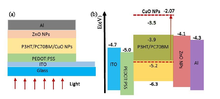
Citation: Aruna P. Wanninayake, Benjamin C. Church, Nidal Abu-Zahra. Effect of ZnO nanoparticles on the power conversion efficiency of organic photovoltaic devices synthesized with CuO nanoparticles[J]. AIMS Materials Science, 2016, 3(3): 927-937. doi: 10.3934/matersci.2016.3.927
[1] | Hai-yan Zhang, Ji-jun Ao, Fang-zhen Bo . Eigenvalues of fourth-order boundary value problems with distributional potentials. AIMS Mathematics, 2022, 7(5): 7294-7317. doi: 10.3934/math.2022407 |
[2] | Haixia Lu, Li Sun . Positive solutions to a semipositone superlinear elastic beam equation. AIMS Mathematics, 2021, 6(5): 4227-4237. doi: 10.3934/math.2021250 |
[3] | Zhanbing Bai, Wen Lian, Yongfang Wei, Sujing Sun . Addendum: Solvability for some fourth order two-point boundary value problems. AIMS Mathematics, 2021, 6(2): 1175-1176. doi: 10.3934/math.2021071 |
[4] | Erdal Bas, Ramazan Ozarslan, Resat Yilmazer . Spectral structure and solution of fractional hydrogen atom difference equations. AIMS Mathematics, 2020, 5(2): 1359-1371. doi: 10.3934/math.2020093 |
[5] | Xiaoping Li, Dexin Chen . On solvability of some $ p $-Laplacian boundary value problems with Caputo fractional derivative. AIMS Mathematics, 2021, 6(12): 13622-13633. doi: 10.3934/math.2021792 |
[6] | Kun Li, Peng Wang . Properties for fourth order discontinuous differential operators with eigenparameter dependent boundary conditions. AIMS Mathematics, 2022, 7(6): 11487-11508. doi: 10.3934/math.2022640 |
[7] | Batirkhan Turmetov, Valery Karachik . On solvability of some inverse problems for a nonlocal fourth-order parabolic equation with multiple involution. AIMS Mathematics, 2024, 9(3): 6832-6849. doi: 10.3934/math.2024333 |
[8] | Erdal Bas, Ramazan Ozarslan . Theory of discrete fractional Sturm–Liouville equations and visual results. AIMS Mathematics, 2019, 4(3): 593-612. doi: 10.3934/math.2019.3.593 |
[9] | Mukhamed Aleroev, Hedi Aleroeva, Temirkhan Aleroev . Proof of the completeness of the system of eigenfunctions for one boundary-value problem for the fractional differential equation. AIMS Mathematics, 2019, 4(3): 714-720. doi: 10.3934/math.2019.3.714 |
[10] | Yanyu Xiang, Aiping Wang . On symmetry of the product of two higher-order quasi-differential operators. AIMS Mathematics, 2023, 8(4): 9483-9505. doi: 10.3934/math.2023478 |
In scientific research and engineering technology, many problems, such as the deformation of engineering building beams and the load of turbine blades under the impact of airflow in fluid mechanics, can be attributed to the existence of solutions of differential equations. And in elastic mechanics and engineering physics, elastic beam is one of the basic components of engineering building. The nonlinear boundary value problem of the fourth order differential equation with different boundary conditions can describes the deflection of elastic beam under external force, the reflects, and the stress. The static beam equation:
y(4)(x)=f(x,y(x)),0<x<1, | (1.1) |
is most studied under the following boundary conditions:
y(0)=y(1)=y″(0)=y″(1)=0, | (1.2) |
or
y(0)=y′(1)=y″(0)=y‴(1)=0, | (1.3) |
where f:[0,1]×[0,∞)→[0,∞) is continuous. They are often used to describe the equilibrium state of the elastic beams. While the problem (1.1), (1.2) describes the static beam with simple support at both ends, the problem (1.1), (1.3) describes the static beam with simple support at one end and sliding support at the other end. These two types of problems, can be converted into second-order equation by simple transformation. Therefore, some methods of studying ordinary differential equations can be applied to the study of problems (1.1), (1.2) and (1.1), (1.3).
The problem (1.1), (1.2) has been investigated in many literutures, see [1,2,3,4,5,6]. Among them, Bai [1] used a new maximum principle to give the solutions for the problem. Gabriele [2] used a local minimum theorem to give the existence of at least one non-trivial solution. Li [3] got the existence of positive solutions based on the fixed point index theory. And Yao [6] used the approximation by operators of completely continuous operator sequence and the Guo-Krasnosel'skii fixed point theorem for cone expansion and compression.
The problem (1.1), (1.3) also has been investigated by many authors, see [7,8,9]. Yao gave the existence of n solutions by choosing suitable cone and using the Krasnosel'skii fixed point theorem in [7]. Yao and Li [8] used the Leray-schauder fixed point theorem to get the existence of positive solutions. Zhao [9] used the fixed point theorem due to Avery-Peterson and Leggett-williams to get the existence of positive solutions. The upper and lower solution method and the fixed-point techniques have been used to study many other problems. We provide reference alone this line for some research on beam equation [10,11].
The typical static elastic beam equation with fixed ends can be described by Eq (1.1) with boundary condition
y(0)=y(1)=y′(0)=y′(1)=0. | (1.4) |
Compared with the above two type problems, this problem can not be solved by directly converting it into some second-order problems. But due to its wide application, many authors set out to find a positive solution to problem (1.1), (1.4). In 1984, Agarwal [12] first considered the problem, and used the compression mapping principle and numerical iteration method to study the existence of solutions. Later, Wu and Ma [13,14] used the Krasnoselskii's fixed point theorem to get the existence results under the following conditions:
(1)¯liml→0min{f(x,v)|(x,v)∈[14,34]×[l24,l]}/l>A;(2)¯liml→∞min14≤x≤34f(x,l)/l>A24. |
Caballero [15] applied a fixed point theorem in partially ordered metric spaces to get a unique symmetric positive solution for problem (1.1), (1.4), where f(x,y) is a nondecreasing function with respect to y for each x∈[0,1], and satisfy the Lipschitz type condition. Obviously the function f(x,y) has strong constraints in above literatures.
This paper study the existence of positive solutions for the following fourth-order two-point boundary value problem:
y(4)(x)=f(x,y(x)),0<x<1, | (1.5) |
y(0)=y(1)=y′(0)=y′(1)=0, | (1.6) |
where f:[0,1]×[0,∞)→[0,∞) is continuous. In section 2, the Green's function is given by the use of the Laplace transform, and some preliminary lemmas also be obtained. In section 3, the eigenvalue of the linear equation corresponding to problem (1.5), (1.6) is given by Ritz method in calculus of variations with the help of the mathematical tool software. The fixed point index value is obtained by using the theory of the self-adjoint operator, and the existence of positive solutions is given by the use of the fixed point index theorem. In section 4, an examples is given to illustrate the main results.
Compared with other literature, in this paper, the way to get the eigenvalue of problem considered is new. We use Laplace transform to get the Green function of this problem, this way is more convenient and easier. And the constraint of f(t,u) in this paper is more weaker than which get in other paper.
For convenience, we introduce some symbols,
ˉf0=¯limy→0+maxx∈[0,1]f(x,y)y,f_0=lim_y→0+minx∈[0,1]f(x,y)y, |
ˉf∞=¯limy→+∞maxx∈[0,1]f(x,y)y,f_∞=lim_y→+∞minx∈[0,1]f(x,y)y. |
Lemma 2.1. Given h∈C[0,1], the unique solution of
y(4)(x)−h(x)=0,0<x<1, | (2.1) |
y(0)=y(1)=y′(0)=y′(1)=0 | (2.2) |
is
y(x)=∫10G(x,s)h(s)ds, | (2.3) |
where
G(x,s)={s2(1−x)2[(x−s)+2(1−s)x]6,0≤s≤x≤1;x2(1−s)2[(s−x)+2(1−x)s]6,0≤x≤s≤1. | (2.4) |
Proof. By the use of Laplace transform on equation (2.1), one has
s4Y(s)−s3y(0)−s2y′(0)−sy″(0)−y‴(0)=H(s), |
where Y(s)=£[y(x)],H(s)=£[h(x)]. Thus,
Y(s)=1s4H(s)+1s4y‴(0)++1s3y″(0)+1s2y′(0)+1sy(0). |
By the use of the inverse Laplace transform and the boundary condition (2.2), one has
y(x)=£−1[Y(s)]=16x3∗h(x)+16x3y‴(0)+12x2y″(0)=16∫x0(x−s)3h(s)ds+16x3y‴(0)+12x2y″(0), | (2.5) |
then
y′(x)=∫x012(x−s)2h(s)ds+12x2y‴(0)+xy″(0). | (2.6) |
Let x=1 in (2.5) and (2.6), then we can get
y″(0)=∫10s(1−s)2h(s)ds, |
y‴(0)=−∫10(1+2s)(1−s)2h(s)ds. |
Put them into Eq (2.5), we get
y(x)=∫x016(x−s)3h(s)ds−∫1016x3(1+2s)(1−s)2h(s)ds+∫1012x2s(1−s)2h(s)ds=∫x016s2(1−x)2[(x−s)+2(1−s)x]h(s)ds+∫1x16x2(1−s)2[(s−x)+2(1−x)s]h(s)ds=∫10G(x,s)h(s)ds. |
The proof is completed.
Remark 2.1. The Green's function (2.4) have been obtained before in some literatures, but to my best knowledge, the way to get it by Laplace transform hadn't been mentioned yet. Obviously, this way is more convenient and easier.
Lemma 2.2. [13] Let a(s):[0,1]→[0,1] define as
G(a(s),s)=max0≤x≤1G(x,s), |
then a(s)=13−2s, for 0≤s≤12;a(s)=21+2s, for 12≤s≤1.
Lemma 2.3. [13] The function G(x,s) defined by (2.4) satisfies:
(i) G(x,s)=G(s,x)>0, for x,s∈[0,1];
(ii) G(x,s)G(a(s),s)≥q(x), where q(x)=min{23x2,23(1−x)2}, for x,s∈[0,1];
(iii) G(x,s)≥124G(a(s),s), for x∈[14,34],s∈[0,1].
Let C+[0,1] be the cone of all nonnegative functions in C[0,1] which is a Banach space with ‖y‖=maxx∈[0,1]|y(x)|. And the cone
D={y∈C+[0,1]|y(x)≥124‖y‖,∀x∈[14,34]}⊂C+[0,1]. |
Then denote
m=min14≤s≤34G(12,s)=34, |
and define T:C+[0,1]→C+[0,1] by
(Ty)(x):=∫10G(x,s)f(s,y(s))ds. | (2.7) |
Lemma 2.4. [13] By Lemma 2.3 and formula (2.7), there holds
(Ty)(x)=∫10G(x,s)f(s,y(s))ds≥q(x)‖Ty‖,x∈[0,1]. |
Lemma 2.5. Let f:[0,1]×[0,∞)→[0,∞) be continuous, then
(1) the operator T:D→D is completely continuous,
(2) the solution of boundary value problem (1.5), (1.6) y(x) satisfies
y(x)≥q(x)‖y‖. |
Proof. The positive solution of problem (1.5), (1.6) is equivalent to the nonzero fixed point of T. On the one hand,
minx∈[14,34](Ty)(x)=minx∈[14,34]∫10G(x,s)f(s,y(s))ds≥124‖Ty‖. |
By the arbitrariness of y and G(x,s)≥0, we obtain T(D)⊂D. Then by the continuity of f and Arzela-Ascoli Theorem, we get (1) holds. On the other hand, by the definition of the operator T and the function a(s), we have
‖Ty‖≤∫10G(a(s),s)f(s,y(s))ds. |
Suppose y∈D is a solution of problem (1.5), (1.6), then
y(x)=(Ty)(x)=∫10G(x,s)f(s,y(s))ds≥q(x)‖Ty‖=q(x)‖y‖. |
The proof is completed.
Given b>0, let
Db={y∈D|y(x)<b}and∂Db={y∈D|y(x)=b}. |
Lemma 2.6. [16] Suppose T:D→D is completely continuous and
(i)infy∈∂Db‖Ty‖>0,
(ii)αTy≠y for ∀y∈∂Db and α≥1.
Then i(T,Db,D)=0.
Lemma 2.7. [16] Suppose T:D→D is completely continuous. If αTy≠y for ∀y∈∂Db and 0<α≤1, then i(T,Db,D)=1.
Lemma 2.8. Assume that G(x,s) is defined as formula (2.4). Then the operator H:C[0,1]→C[0,1],
(Hz)(x)=∫10G(x,s)z(s)ds, |
is a self-adjoint operator.
Proof. By Lemma 2.1, it is clear that G(x,s) is a real symmetric function, that is to say that, G(x,s)=G(s,x) for 0≤s,x≤1. Thus, for ∀z1=z1(s),z2=z2(s)∈C[0,1], there holds
(Hz1,z2)=∫10(Hz1)(x)z2(x)dx=∫10∫10G(x,s)z1(s)z2(x)dsdx=∫10z1(s)∫10G(x,s)z2(x)dxds=∫10z1(s)∫10G(s,x)z2(x)dxds=∫10z1(s)(Hz2)(s)ds=(z1,Hz2). |
So, the operator H is a self-adjoint operator.
Lemma 3.1. The first eigenvalue λ1 of the problem
y(4)(x)−λy(x)=0, | (3.1) |
y(0)=y(1)=y′(0)=y′(1)=0, | (3.2) |
is λ1≈500.564.
Proof. Define the linear differential operator L:{y∈C4[0,1]∣y(0)=y(1)=y′(0)=y′(1)=0}→C[0,1] as
(Ly)(x)=y(4)(x). | (3.3) |
With Ritz method, the problem which to get the first eigenvalue λ1 can be transformed to get the extreme value of the functional
J[y]=∫10yLydx=∫10y(x)[y(4)(x)]dx, | (3.4) |
under the normalization condition
∫10y2(x)dx=1. | (3.5) |
Combing the definition of the functional J and the boundary condition (3.2), one has
J[y]=∫10y(x)[y(4)(x)]dx=∫10[y″(x)]2dx. |
Choose the primary function as
yk(x)=(1−x)2x2k,(k=1,2,3,⋯), |
then, the n-th order approximate solution of the functional extremum function is
yn(x)=x2(1−x)2(a1+a2x+⋯+anxn−1). | (3.6) |
By (3.4), (3.5), there is
J[yn(x)]=∫10[y″n(x)]2dx, | (3.7) |
∫10y2n(x)dx=1. | (3.8) |
Then the Lagrangian function
F(a1,a2,⋯,an,τ)=J[yn(x)]+τ[∫10y2n(x)dx−1]=∫10[y″n(x)]2dx+τ[∫10y2n(x)dx−1]. |
Now, we solve the following equation system by the use of the mathematical tool software Mathematica,
∂F∂ai=0(i=1,2,3,⋯,n),and∂F∂τ=0. |
Firstly, we get ai(i=1,2,3,⋯,n) and τ, then, plug them into (3.6) to get yn(x). By Eq (3.7) we get the corresponding eigenvalue λ1=J[yn(x)]≈500.564 for n≥6. The proof is completed.
Remark 3.1. Although some authors mentioned the eigenvalue before, but to my best knowledge, the eigenvalue of problem (3.1), (3.2) hadn't been obtained yet. However, we use the Ritz-Method to get the concrete eigenvalue λ1 here.
Theorem 3.1. Suppose one of the following relation is true:
(i) ˉf0<λ1, f_∞>λ1;
(ii) f_0>λ1,ˉf∞<λ1.
Then boundary value problem (1.5), (1.6) has at least one positive solution.
Proof. (i) By ˉf0<λ1, for ϵ∈(0,λ1), there exists b0>0 such that
f(x,y)≤(λ1−ϵ)y,∀x∈[0,1],y∈[0,b0]. | (3.9) |
Set b∈(0,b0). Assume there exist y0∈∂Db and α0∈(0,1] such that α0Ty0=y0. Then y0 satisfies
y(4)0(x)=α0f(x,y0(x)),0≤x≤1. | (3.10) |
Taking into account (3.9) and (3.10), there is
y(4)0(x)=α0f(x,y0(x))≤α0(λ1−ϵ)y0(x)≤(λ1−ϵ)y0(x). |
Due to the fact that the inverse operator of a self-adjoint operator is self-adjoint and Lemma 2.8, the operator L defined by (3.3) is a self-adjoint operator. Suppose ˆy∈D is a eigenfunction of L with respect to λ1 such that ∫10ˆy(x)dx=1, that is to say that
Lˆy=λ1ˆy. |
Then
(Ly0,ˆy)=(y0,Lˆy)=(y0,λ1ˆy)=λ1(y0,ˆy). |
So we get
λ1(y0,ˆy)≤(λ1−ϵ)(y0,ˆy). |
obviously this is a contradictory. Hence Lemma 2.7 yields that
i(T,Db,D)=1. | (3.11) |
Since f_∞>λ1, for given ϵ>0, there exists K>0 such that
f(x,y)≥(λ1+ϵ)y,∀x∈[0,1],y≥K, | (3.12) |
suppose C=max0≤x≤1,0≤y≤K|f(x,y)−(λ1+ϵ)y|+1, then
f(x,y)≥(λ1+ϵ)y−C,∀x∈[0,1],y∈[0,+∞). |
Let r>r0:=max{24K,b0}. For y∈∂Dr, there is y(s)≥124‖y‖>K for s∈[14,34], then, by (3.12)
‖Ty‖≥(Ty)(12)=∫10G(12,s)f(s,y(s))ds≥∫3414m(λ1+ϵ)y(s)ds≥124∫3414m(λ1+ϵ)‖y‖ds≥148m(λ1+ϵ)‖y‖ | (3.13) |
So infy∈∂Dr‖Ty‖>0.
Suppose there exist y0∈Dr and μ0≥1 such that μ0Ty0=y0, then
(Ly0)(x)=μ0f(x,y0(x))≥(λ1+ϵ)y0(x)−C. |
Thus,
λ1(y0,ˆy)=(y0,λ1ˆy)=(y0,Lˆy)=(Ly0,ˆy)≥(λ1+ϵ)(y0,ˆy)−C. |
So,
(y0,ˆy)≤Cϵ. |
Similar to the proof of Lemma 2.5, by μ0Ty0=y0, one has
y0(x)≥(Ty0)(x)≥q(x)‖y0‖. |
So,
(y0,ˆy)≥‖y0‖∫10q(x)ˆy(x)dx. |
Thus,
‖y0‖≤Cϵ[∫10q(x)ˆy(x)dx]−1:=ˉr. | (3.14) |
Now set r>max{ˉr,b0}, then there is μTy≠y for ∀y∈∂Dr and μ≥1. Consequently, two conditions of Lemma 2.6 all hold, thus
i(T,Dr,D)=0. | (3.15) |
By (3.11) and (3.15) there is
i(T,Dr∖¯Db,D)=i(T,Dr,D)−i(T,Db,D)=−1. | (3.16) |
Hence T has a fixed point in Dr∖¯Db.
(ii) Since f_0>λ1, for ϵ>0, there exists h0>0 such that
f(x,y)≥(λ1+ϵ)y,∀x∈[0,1],0≤y≤h0. | (3.17) |
Set h∈(0,h0), similar to (3.13), one has
‖Ty‖≥148m(λ1+ϵ)‖y‖,∀y∈∂Dh, |
so infy∈∂Db‖Ty‖>0.
Assume there exist y1∈∂Dh and α1≥1 such that α1Ty1=y1, then
λ1(y1,ˆy)=(y1,λ1ˆy)=(y1,Lˆy)=(Ly1,ˆy)≥(λ1+ϵ)(y1,ˆy). |
Obviously this is a contradiction, because (y1,ˆy)>0. Therefore, Lemma 2.5 yields that
i(T,Dh,D)=0. | (3.18) |
On the other hand, since ˉf∞<λ1, for ϵ∈(0,λ1), there exists K2>0 such that
f(x,y)≤(λ1−ϵ)y,∀x∈[0,1],y≥K2. |
Let C=max0≤x≤1,0≤y≤K2|f(x,y)−(λ1−ϵ)y|+1, then
f(x,y)≤(λ1−ϵ)y+C,∀x∈[0,1],y∈[0,+∞). | (3.19) |
Assume there exist y2∈D and α2∈(0,1] such that α2Ty2=y2, then
λ1(y2,ˆy)=(y2,λ1ˆy)=(y1,Lˆy)=(Ly1,ˆy)≤(λ1−ϵ)(y2,ˆy)+C. |
Similar to the previous proof, one has ‖y2‖≤ˉr. Set r>max{ˉr,h0}, we get αTy≠y for ∀y∈∂Dr and α∈(0,1]. Hence by Lemma 2.7,
i(T,Dr,D)=1, | (3.20) |
then
i(T,Dr∖¯Db,D)=i(T,Dr,D)−i(T,Db,D)=1. |
In conclusion, the boundary value problem (1.5), (1.6) has at least one positive solution.
Remark 3.2. Compared with literatures [14,15] and so on, the constraint of f(x,y) in our results is weaker.
Example 4.1. Consider the problem:
y(4)(x)=[y(x)]θ+(300−x)y(x),0<x<1,θ≠1, | (4.1) |
y(0)=y(1)=y′(0)=y′(1)=0. | (4.2) |
It's obviously that f(x,y)y=yθ−1+300−x.
Case (1): θ>1, there are
(i)ˉf0=¯limy→0+maxx∈[0,1]f(x,y)y=300<500.564≊λ1;(ii)f_∞=lim_y→+∞minx∈[0,1]f(x,y)y=+∞>500.564≊λ1, |
Case (2): θ<1, there are
(i)f_0=lim_y→0+minx∈[0,1]f(x,y)y=+∞>500.564≊λ1;(ii)ˉf∞=¯limy→+∞maxx∈[0,1]f(x,y)y=300<500.564≊λ1, |
By Theorem 3.1, for θ≠1, Problem (4.1), (4.2) has at least one positive solution.
The fourth order differential equations have been applied in different aspects of applied mathematics and physics, especially in the theory of elastic beams and stability. In this paper, the fourth-order two-point boundary value problem is studied, which can describe some changes when the elastic beam deforms or rotates when it is subjected to external forces, and provides an important theoretical basis for solving the problem. And compare with other literature, our method in this paper makes the equation more widely used and describes the equilibrium state of the elastic beam better.
This work is supported by Natural Science Foundation of China (Grant No.11571207), the Taishan Scholar project, and SDUST graduate innovation project SDKDYC190237.
The authors declare no conflict of interest in this paper.
[1] | Dang MT, Hirsch L, Wantz G (2011) Best Seller in Polymer Photovoltaic Research. Adv Mater 23: 3597–3602. |
[2] |
Wang PH, Lee HF, Huang YC, et al. (2014) The Proton Dissociation Constant of Additive Effect on Self-Assembly of Poly(3-hexyl-thiophene) for Organic Solar Cells, Electron. Mater Lett 10: 767–773. doi: 10.1007/s13391-013-3274-0
![]() |
[3] |
Zhang F, Mammo W, Andersson LM, et al. (2006) Low-Bandgap Alternating Fluorene Copolymer/Methanofullerene Heterojunctions in Efficient Near-Infrared Polymer Solar Cells. Adv Mater 18: 2169–2173. doi: 10.1002/adma.200600124
![]() |
[4] | Huang Y, Guo X, Liu F, et al. (2012) Improving the Ordering and Photovoltaic Properties by Extending–Conjugated Area of Electron-Donating Units in Polymers with D-A Structure. Adv Mater 24: 3383–3389. |
[5] | Wang E, Tao L, Wang Z, et al. (2010) An Easily Synthesized Blue Polymer for High-Performance Polymer Solar Cells. Adv Mater 22: 5240–5244. |
[6] | Reese M.O., Nardes A.M., Rupert B.L., et al. (2010) Photoinduced Degradation of Polymer and Polymer–Fullerene Active Layers: Experiment and Theory. Adv Funct Mater 20: 3476–3483. |
[7] | He Z, Mei Z, Su S, et al. (2012) Enhanced power-conversion efficiency in polymer solar cells using an inverted device structure. Nature Photon 6: 591–595. |
[8] | Shao S, Liu J, Zhang B, et al. (2011) Enhanced stability of zinc oxide-based hybrid polymer solar cells by manipulating ultraviolet light distribution in the active layer. Appl Phys Lett 98: 203304–203307. |
[9] |
Huang J, Yin Z, Zheng Q (2011) Applications of ZnO in organic and hybrid solar cells. Energy Environ Sci 4: 3861–3877. doi: 10.1039/c1ee01873f
![]() |
[10] | Lin Y-Y, Chu T-H, Li S-S, et al. (2009) Interfacial Nanostructuring on the Performance of Polymer/TiO2 Nanorod Bulk Heterojunction Solar Cells. J Am Chem Soc 131: 3644–3649. |
[11] |
Sekine N, Chou CH, Kwan WL, et al. (2009) ZnO nano-ridge structure and its application in inverted polymer solar cell. Org Electron 10: 1473–1477. doi: 10.1016/j.orgel.2009.08.011
![]() |
[12] |
Oh SA, Heo SJ, Yang JS, et al. (2013) Effects of ZnO Nanoparticles on P3HT:PCBM Organic Solar Cells with DMF-Modulated PEDOT:PSS Buffer Layers. ACS Appl Mater Interfaces 5: 11530–11534. doi: 10.1021/am4046475
![]() |
[13] | Wu Z, Song T, Xia Z, et al. (2013) Enhanced performance of polymer solar cell with ZnO nanoparticle electron transporting layer passivated by in situ cross-linked three-dimensional polymer network. Nanotechnology 24: 484012. |
[14] | Zhu F, Chen X, Lu Z, et al. (2014) Efficiency Enhancement of Inverted Polymer Solar Cells Using Ionic Liquid-functionalized Carbon Nanoparticles-modified ZnO as Electron Selective Layer. Nano-Micro Lett 6: 24–29. |
[15] |
Gao HL, Zhang XG, Meng JH, et al. (2015) Enhanced efficiency in polymer solar cells via hydrogen plasma treatment of ZnO electron transport layers. J Mater Chem A 3: 3719–3725. doi: 10.1039/C4TA05541A
![]() |
[16] |
Iwan A, Palewicz M, Tazbir I, et al. (2016) Influence of ZnO:Al, MoO3 and PEDOT:PSS on efficiency in standard and inverted polymer solar cells based on polyazomethine and poly(3-hexylthiophene). Electrochimica Acta 191: 784–794. doi: 10.1016/j.electacta.2016.01.107
![]() |
[17] | Wanninayake A, Gunashekar S, Li S, et al. (2015) Performance enhancement of polymer solar cells using copper oxide nanoparticles. Semicond Sci Technol 30: 064004. |
[18] | Wanninayake AP, Gunashekar S, Li S, et al. (2015) CuO Nanoparticles Based Bulk Heterojunction Solar Cells: Investigations on Morphology and Performance. J Sol Energy Eng 137: 031016. |
[19] | Kidowaki H, Oku T, Akiyama T (2012) Fabrication and characterization of CuO/ZnO solar cells. J Phys Conf Ser 352: 012022. |
[20] |
Ikram M, Murrayc R, Imran M, et al. (2016) Enhanced performance of P3HT/ (PCBM: ZnO: TiO2) blend based hybrid organic solar cells. Mater Res Bull 75: 35–40. doi: 10.1016/j.materresbull.2015.11.031
![]() |
[21] |
Ikram M, Murray R, Hussain A, et al. (2014) Hybrid organic solar cells using both ZnO and PCBM as electron acceptor materials. Mater Sci Eng B 189: 64–69. doi: 10.1016/j.mseb.2014.08.005
![]() |
[22] |
Qian L, Yang J, Zhou R, et al. (2011) Hybrid polymer-CdSe solar cells with a ZnO nanoparticle buffer layer for improved efficiency and lifetime. J Mater Chem 21: 3814–3817. doi: 10.1039/c0jm03799k
![]() |
[23] |
Wang M, Wang X (2008) P3HT-ZnO bulk-heterojunction solar cell sensitized by a perylene derivative. Sol Energy Mater Sol Cells 92: 766–771. doi: 10.1016/j.solmat.2008.01.015
![]() |
[24] |
Beek WJE, Wienk MM, Janssen RAJ (2006) Hybrid Solar Cells from Regioregular Polythiophene and ZnO Nanoparticles. Adv Funct Mater 16: 1112–1116. doi: 10.1002/adfm.200500573
![]() |
[25] | Ochiai S, Kumar P, Santhakumar K, et al. (2013) Examining the Effect of Additives and Thicknesses of Hole Transport Layer for Efficient Organic Solar Cell Devices. Electron Mater Lett 9: 399–403. |
[26] |
Kim JY, Kim SH, Lee HH, et al. (2006) New Architecture for High-Efficiency Polymer Photovoltaic Cells Using Solution-Based Titanium Oxide as an Optical Spacer. Adv Mater 18: 572–576. doi: 10.1002/adma.200501825
![]() |
[27] | Roest L, Kelly JJ, Vanmaekelbergh D, et al. (2002) Staircase in the Electron Mobility of a ZnO Quantum Dot Assembly due to Shell Filling. Phys Rev Lett 89: 036801. |
[28] |
Ikram M, Ali S, Murray R, et al. (2015) Influence of fullerene derivative replacement with TiO2nanoparticles in organic bulk heterojunction solar cells. Curr Appl Phys 15: 48–54. doi: 10.1016/j.cap.2014.10.026
![]() |
[29] |
Djara V, Bernède J (2005) Effect of the interface morphology on the fill factor of plastic solar cells. Thin Solid Films 493: 273–277. doi: 10.1016/j.tsf.2005.06.098
![]() |
[30] |
Oo T, Mathews N, Tam T, et al. (2010) Investigation of photophysical, morphological and photovoltaic behavior of poly (p-phenylene vinylene) based polymer/oligomer blends. Thin Solid Films 518: 5292–5299. doi: 10.1016/j.tsf.2010.04.115
![]() |
[31] | Ji CH, Oh IS, Oh SY (2015) Improving the performance of organic solar cells using an electron transport layer of B4PyMPM self-assembled nanostructures. Electron Mater Lett 11: 795–800. |
[32] |
Shahini A, Abbasian K (2012) Charge carriers and excitons transport in an organic solar cell-theory and simulation. Electron Mater Lett 8: 435–443. doi: 10.1007/s13391-012-2021-2
![]() |
1. | Yanhong Zhang, Li Chen, Positive solution for a class of nonlinear fourth-order boundary value problem, 2023, 8, 2473-6988, 1014, 10.3934/math.2023049 | |
2. | Lucía López-Somoza, F. Adrián F. Tojo, Asymptotic properties of PDEs in compact spaces, 2021, 23, 1661-7738, 10.1007/s11784-021-00905-w | |
3. | Khudija Bibi, Solutions of initial and boundary value problems using invariant curves, 2024, 9, 2473-6988, 22057, 10.3934/math.20241072 | |
4. | Nikolay D. Dimitrov, Jagan Mohan Jonnalagadda, Existence of Three Positive Solutions for Boundary Value Problem of Fourth Order with Sign-Changing Green’s Function, 2024, 16, 2073-8994, 1321, 10.3390/sym16101321 | |
5. | Abdissalam Sarsenbi, Abdizhahan Sarsenbi, Boundary value problems for a second-order differential equation with involution in the second derivative and their solvability, 2023, 8, 2473-6988, 26275, 10.3934/math.20231340 | |
6. | Xinyuan Pan, Xiaofei He, Aimin Hu, EXISTENCE AND NONEXISTENCE OF SOLUTIONS FOR A CLASS OF p-LAPLACIAN-TYPE FRACTIONAL FOUR-POINT BOUNDARY-VALUE PROBLEMS WITH A PARAMETER, 2023, 53, 0035-7596, 10.1216/rmj.2023.53.1537 |