
Citation: Joachim P Sturmberg, Geoff M McDonnell. How Modelling could Contribute to Reforming Primary Care—Tweaking “the Ecology of Medical Care” in Australia[J]. AIMS Medical Science, 2016, 3(3): 298-311. doi: 10.3934/medsci.2016.3.298
[1] | Martin Heida . Stochastic homogenization on perforated domains Ⅰ – Extension Operators. Networks and Heterogeneous Media, 2023, 18(4): 1820-1897. doi: 10.3934/nhm.2023079 |
[2] | Martin Heida, Benedikt Jahnel, Anh Duc Vu . Regularized homogenization on irregularly perforated domains. Networks and Heterogeneous Media, 2025, 20(1): 165-212. doi: 10.3934/nhm.2025010 |
[3] | Hakima Bessaih, Yalchin Efendiev, Florin Maris . Homogenization of the evolution Stokes equation in a perforated domain with a stochastic Fourier boundary condition. Networks and Heterogeneous Media, 2015, 10(2): 343-367. doi: 10.3934/nhm.2015.10.343 |
[4] | Luca Lussardi, Stefano Marini, Marco Veneroni . Stochastic homogenization of maximal monotone relations and applications. Networks and Heterogeneous Media, 2018, 13(1): 27-45. doi: 10.3934/nhm.2018002 |
[5] | Patrick Henning . Convergence of MsFEM approximations for elliptic, non-periodic homogenization problems. Networks and Heterogeneous Media, 2012, 7(3): 503-524. doi: 10.3934/nhm.2012.7.503 |
[6] | Nils Svanstedt . Multiscale stochastic homogenization of monotone operators. Networks and Heterogeneous Media, 2007, 2(1): 181-192. doi: 10.3934/nhm.2007.2.181 |
[7] | Brahim Amaziane, Leonid Pankratov, Andrey Piatnitski . Homogenization of variational functionals with nonstandard growth in perforated domains. Networks and Heterogeneous Media, 2010, 5(2): 189-215. doi: 10.3934/nhm.2010.5.189 |
[8] | Peter Bella, Arianna Giunti . Green's function for elliptic systems: Moment bounds. Networks and Heterogeneous Media, 2018, 13(1): 155-176. doi: 10.3934/nhm.2018007 |
[9] | Iryna Pankratova, Andrey Piatnitski . Homogenization of convection-diffusion equation in infinite cylinder. Networks and Heterogeneous Media, 2011, 6(1): 111-126. doi: 10.3934/nhm.2011.6.111 |
[10] | Valeria Chiado Piat, Sergey S. Nazarov, Andrey Piatnitski . Steklov problems in perforated domains with a coefficient of indefinite sign. Networks and Heterogeneous Media, 2012, 7(1): 151-178. doi: 10.3934/nhm.2012.7.151 |
Let p(ω)⊂Rd be a stationary ergodic connected random open set with random variable ω and let ε>0 be the smallness parameter. The concept of stationary ergodic random open sets was introduced in detail in Part I [5], and we will give a simplified version below, which focuses on the properties used in the present Part III.
For a bounded open domain Q, we then consider pε(ω)=εp(ω), Qεp(ω):=Q∩pε(ω) and Γε(ω):=Q∩∂pε(ω) with outer normal νΓε(ω). In order to simplify notation, we keep in mind that p and Qεp are random variables and drop the explicit writing of ω.
Denoting W1,p0,∂Q(Qεp):={u∈W1,p(Qεp):u|∂Q≡0} one would classically be interested in a family of extension operators Uε:W1,p0,∂Q(Qεp)→W1,p(Q) such that for some C independent from ε it holds
‖∇Uεu‖Lp(Q)≤C‖∇u‖Lp(Qεp),‖Uεu‖Lp(Q)≤C‖u‖Lp(Qεp). | (1.1) |
However, estimates of the form Eq (1.1) are known to exist only for (global) John domains but from Part I we know that even random Lipschitz domains are mostly not (globally) John. We recall the definition of a John domain and refer to Figure 1 for an illustration of issues arising in the context of infinite random geometries:
Definition (John domains). A bounded domain P⊂Rd is a John domain if there exists ε,δ>0 s.t. for every x,y∈P with |x−y|<δ there exists a rectifiable path γ:[0,1]→P from x to y with
lengthγ≤1ε|x−y|and | (1.2) |
∀t∈(0,1):infz∈Rd∖P|γ(t)−z|≥ε|x−γ(t)||γ(t)−y||x−y|. | (1.3) |
On the other hand Part I [5] gives rise to the hope that we can find 1≤r<p and a family of extension operators Uε:W1,p0,∂Q(Qεp)→W1,r(Q) for scalar valued functions resp. Uε:W1,p0,∂Q(Qεp)→W1,r(Rd) for vector valued functions such that
1|Q|∫Rd|∇Uεu|r≤(C|Q|∫Q∩εp|∇u|p)rp,1|Q|∫Rd|Uεu|r≤(C|Q|∫Q∩εp|u|p)rp, | (1.4) |
where the full support of Uεu lies within Bεβ(Q) for ε small enough and some fixed β∈(0,1) depending on p.
In Part I we have established a general abstract framework for the derivation of uniform bounds on extension operators and except for two special examples, the results in Part I are rather vague, missing a general theory to deal with the connectivity of the domain. The connectivity for general geometries will be the main topic of the present work. We note at this point that connectivity is also the major issue for other former works to restrict to inclusions of an absolutely bounded diameter [3,10]. Our method of proof, based on Part I, is different from other proofs in the literature, particularly the literature for periodic [7] or John [2,8] domains, even though some patterns recur such as the construction of suitable paths along overlapping sets of an open covering. For a further overview over the history and the literature, the reader is referred to Parts I and II [6].
Let us finally note that replacing Eq (1.1) by Eq (1.4) also affects the analysis in the homogenization process and we refer to Part II [6] where this has been discussed.
Throughout this work, we use (ei)i=1,…d for the Euclidean basis of Rd. Given a metric space (M,d) we denote Br(x) the open ball around x∈M with radius r>0. The surface of the unit ball in Rd is Sd−1. Furthermore, we denote
∀A⊂Rd:Br(A):=⋃x∈ABr(x). |
A sequence of points will be labeled by x:=(xi)i∈N.
In what follows, we will assume that p=p(ω) is also a random connected domain, that is Lipschitz for almost every realization. We formally introduce the concepts of stationarity and ergodicity of stochastic processes in Section 2.4. If no confusion occurs, we drop (ω) in the notation wherever possible in order to improve readability.
According to Part I Chapter 3 for every stationary ergodic random open set p the following can be established.
Lemma 1.1. Let p be a stationary ergodic random open set. Then there exists r>0 and a positive, monotonically decreasing functions fP with fP(R)→0 as R→∞ and a random point process xr=(xa)a∈N jointly stationary with p such that
● Br2(xr)⊂p,
● for all a,b∈N, a≠b, it holds |xa−xb|>2r,
● P(BR(0)∩xr=∅)≤fP(R).
Jointly stationary in the sense of Part I means that both of the joint distributions of xr and p are invariant over all shifts x∈Rd or over all shifts x∈2rZd. Constructing from xr=(xa)a∈N a Voronoi tessellation of cells (Ga)a∈N of diameter da=d(xa):=supx,y∈Ga|x−y|, then according to Part I for some constant C≥1
P(d(xa)>D)<fd(D):=CfP(C−1D). | (1.5) |
Furthermore, for any x∈xr and y∈p let
Υ(x,y):={γ:[0,1]→p|γ∈C([0,1];p), γ(0)=x,γ(1)=y} |
denote the set of all continuous paths from x to y inside p. Given x∈xr we further denote
R(x):=r+inf{R>r: ∀y∈B5d(x)(x)∃γ∈Υ(x,y):γ([0,1])⊂BR(x)}. | (1.6) |
Connectedness ensures R(x)<∞ for every x∈xr. Denoting S(x):=R(x)/d(x) we consider monotonically decreasing functions fS,fR:[0,∞)→R given through
fR(R):=P(R(xa)>R),fS(S):=P(S(xa)>S). | (1.7) |
We call R the connectivity radius and S the stretch factor.
Definition 1.2 (Local (δ,M)-Regularity). The domain p⊂Rd is called (δ,M)-regular in p0∈∂p if there exists an open set U⊂Rd−1 and a Lipschitz continuous function ϕ:U→R with Lipschitz constant greater or equal to M such that ∂p∩Bδ(p0) is subset of the graph of the function φ:U→Rd,˜x↦(˜x,ϕ(˜x)) in some suitable coordinate system.
Definition 1.3. For a stationary random Lipschitz domain p⊂Rd with r from Lemma 1.1 and for every p∈∂p and n∈N∪{0}
δr(p):=12supδ<2r{∃M>0:p is (δ,M)-regular in p}, | (1.8) |
MR(p):=infη>Rinf{M:p is (η,M)-regular in p}, | (1.9) |
ρn(p):=supR<δ(p)r(4MR(p)2+2)−n2, | (1.10) |
For every p∈∂p it holds that
R2>R1impliesMR2(p)≥MR1(p). |
Since no confusion occurs, we write δ=δr for simplicity.
Definition 1.4 (Extension order). The geometry is of extension order n∈N∪{0} if there exists C>0 such that for almost every p∈∂p there exists a local extension operator
Un:W1,p(B18δ(p)(p)∩p)→W1,p(B18ρn(p)(p)),‖∇Unu‖Lp(B18ρn(p)(p))≤C(1+M18δ(p)(p))‖∇u‖Lp(B18δ(p)(p)). | (1.11) |
In particular, we assume that n∈N and C>0 in the above definition are deterministic and global. Part I shows that every locally Lipschitz geometry is of extension order n=1 and C is independent from the geometry, though better values (i.e., n = 0) for n are possible for some geometries. A random distribution of n among the values 0 and 1 could be handled within the theory developped in Part I and in the present paper, but this would lead to additional effort in notation and presentation with no additional insight.
Definition 1.5 (Inner microscopic regularity, see Figure 2). Given n∈N and ˜ρ:=2−5ρn, the inner microscopic regularity α∈[0,1] is
α:=inf{˜α≥0:∀p∈∂p∃y∈p:B˜ρ(p)/32(1+M˜ρ(p)(p)˜α)(y)⊂B˜ρ(p)/8(p)∩p}. |
As demonstrated in Part I, the values of α and n as well as the distribution of M and ρn are crucial for the validity of Eq (1.4) for a given pair (r,p).
We find the following main result.
Theorem 1.6. Let Q⊂Rd be a bounded Lipschitz domain. Let p(ω) be a stationary ergodic random connected open set in Rd of extension order n and with inner microscopic regularity α. Furthermore let xr be a jointly stationary point process satisfying Assumption 1.1. Given constants 1≤r<s<p and q,˜q∈[1,∞) with sp+1q+sr˜q=1 and writing
Pk,R:=P(forx∈xr:d(x)∈[k,k+1),R(x)∈[R,R+1)) |
let the following hold for sr:=s(r+1)−rr:
E1=∞∑k,R=1(k+1)d(q+1)+3drq+r(q−1)(R+1)d(q+1)+srq+r(q−1)Pk,R<∞, | (1.12) |
E2=E(δ(1+M3δ4)pp−r[(n+α)(d−1)+r]+d−2)<∞, | (1.13) |
E3=E(˜ρ(1−d)(r˜q−1)+2+dn˜Mαd+d−24˜ρn)<∞. | (1.14) |
Alternatively let d and S be independent and writing
Pd,k:=P(forx∈xr:d(x)∈[k,k+1))PS,S:=P(forx∈xr:S(x)∈[S,S+1)) |
replace condition Eq(1.12) with
E4=∞∑k,S=1(k+1)d(q+1)+d(3r+sr)q+r(q−1)(S+1)d(q+1)+dsrq+r(q−1)<∞. | (1.15) |
Then there exists β0∈(0,1) not depending on ω such that for almost every ω there exists an extension operator Uω:W1,ploc(p(ω))→W1,rloc(Rd) and a constant Cω and N0≥1 such that for every N>N0 it holds
1|NQ|∫NQ|∇Uωu|r≤Cω(1|NQ|∫p(ω)∩BNβ0(NQ)|∇u|p)rp, | (1.16) |
1|NQ|∫NQ|Uωu|r≤Cω(1|NQ|∫p(ω)∩BNβ0(NQ)|u|p)rp. | (1.17) |
Remark 1.7. Of course it is desireable to get moment estimates on Cω but there is a problem involved here: On one hand, Cω is clearly related to E1, ... E4. However, for a given fixed N there arises the following type of inequality in the proofs which is clearly related to E3:
1|NQ|∫NQ|∇Uωu|r≤(1|NQ|∫p(ω)∩BNβ0(NQ)˜ρ(1−d)(r˜q−1)+2+dn˜Mαd+d−24˜ρn)p−rp⋅…⋯⋅(1|NQ|∫p(ω)∩BNβ0(NQ)|∇u|p)rp+… |
and similar terms appear for E1, E2 and E4. Now the first bracket on the right hand side converges to a positive number by the ergodic theorem. However, for our given ω it may become very large with its maximum being not related to E3 or ω in a currently quantifyable way. On the other hand, if u=u(x,ω) is a random function and we go back to the very begining of Part I, averaging over Ω in all calculations, we could get the following:
E1|NQ|∫NQ|∇Uωu|r≤C(E1+E2+E3)p−rp(E1|NQ|∫p(ω)∩BNβ0(NQ)|∇u|p)rp. |
with C not depending on ω or N.
Remark 1.8. Observe that we do not impose bounds on δ−1 because the above formula already contains bounds on ρ−1. Through the formula δ−1∝ρ−1(1+M) we can replace the bounds on ρ−1 by bounds on δ−1 and vice versa.
Remark 1.9. Theorem 1.6 shows that if the distribution of δ, M, d, S is good enough, we can have any r<p. Finally, if δ is bounded away from 0 and M, d, S are uniformly bounded from above, we are back in the minimally smooth setting which allows r=p.
We may apply a rescaling N=ε−1 for some ε>0. Writing
[Uεωu](x):=[Uωu(ε⋅)](xε) |
inequality (1.16) reads
1|Q|∫Q|Uεωu|r≤Cω(1|Q|∫[εp(ω)]∩Bε1−β0(Q)|∇u|p)rp. |
The important insight is that χBε1−β0(Q)→χQ in Lp(Rd) for any 1≤p<∞ and hence in the limit Uεωu is determined mostly by the values of u(x) for x∈Q. Moreover it was shown in Part I that u|(εp)∩∂Q≡0 implies that the support of Uεωu will ultimately reduce to Q in the limit.
Theorem 1.6 has a rather broad range of geometries it may be applied to. It also gives a hint how probabilistic construction of random geometries might be modified to ensure the existence of extension operators. One particular question that the author was asked frequently on seminar talks and workshops is the applicability of the above result to the boolean model treated in Part I. This is a geometry constructed by assigning to a family of random points balls with radius 1 around these points. The above result is then applicable if the probability of "touching", i.e., the boundaries of two balls meet in precisely 1 point, has probability zero and the distribution of "small overlap" and "small distance" of two different balls is sufficiently small. We refer to Section 6 of Part I where such a calculation is carried out in detail.
In Section 2 we collect some results from Part I and modify the Voronoi integration lemma from there including a new and shortened proof. In Section 3 we prove Theorem 1.6 based on one of the main results from Part I. An outline of the proof is provided at the beginning of Section 3.
The constant C on the right hand side of Eq (1.16) depends on averaged weights of δ, M, da, Sa and Ra related to Eqs (1.12)–(1.15). In order to judge whether these averages are bounded as n→∞, we will rely on the integration theory that is recalled below. In particular, this theory is connected to the ergodic theorems and the Palm measure. We start by briefly explaining how the following results will be applied later on.
In Section 2.1 we recall η-regularity introduced in Part I. This concept allows us to cover any closed sets by a suitable family of open balls such that the covering is locally finite and uniformly bounded by a constant. While in Part I this was used to cover only the boundary of p in terms of ρn, we will later in Section 3.3 use this result to extend the covering to the interior full domain.
In Section 2.2 we construct from (δ,M) (notably only defined on ∂p) various integrable functions on Rd which are denoted e.g., ρ[…],Rd, δ[…],Rd, M[…],Rd. However, we emphasize at this point that the distribution of ρn(x), δ(x) or M(x) are w.r.t. the condition that x∈∂p(ω). Hence, it is necessary to control integrals over the functions ρ[…],Rd, δ[…],Rd, M[…],Rd by integrals over the functions ρn(x), δ(x) or M(x), which leads to Lemma 2.6.
Section 2.3 provides a frequently used Poincaré inequality and in Section 2.4 we introduce the ergodic theorems on p and ∂p which will ensure that all the above mentioned averaging integrals converge to their expectation as the support grows infinitely large.
Finally in Section 2.5 we study functions
b(y):=∑x∈XrχBR(x)(x)(x)d(x)ηR(x)ξ, |
and provide an estimate on the expectation of bq, q∈[1,∞). This will help us to control integrals that enter the constant C from the mesoscopic geometric properties.
We summarize the concept of η-regularity and its major consequences from Part I. Note that Lemma 2.2 was proved in Part I only for Γ=∂p. However, the only property of ∂p used for the proof is its closedness.
Definition 2.1 (η- regularity). Let Γ be a closed set. For a function η:Γ→(0,r] we call Γη-regular if
∀p∈Γ,ε∈(0,12),˜p∈Bεη(p)(p)∩Γ:η(˜p)>(1−ε)η(p). | (2.1) |
Lemma 2.2. Let Γ be a locally η-regular set for η:Γ→(0,r). Then η:p→R is locally Lipschitz continuous with Lipschitz constant 1 and for every ε∈(0,12) and ˜p∈Bεη(p)∩Γ it holds
1−ε1−2εη(p)>η(˜p)>η(p)−|p−˜p|>(1−ε)η(p), | (2.2) |
|p−˜p|≤εmax{η(p),η(˜p)}⇒|p−˜p|≤ε1−εmin{η(p),η(˜p)}. | (2.3) |
Theorem 2.3. Let Γ⊂Rd be a closed set and let η(⋅)∈C(Γ) be bounded and satisfy for every ε∈(0,12) and for |p−˜p|<εη(p)
1−ε1−2εη(p)>η(˜p)>η(p)−|p−˜p|>(1−ε)η(p). | (2.4) |
and define ˜η(p)=2−Kη(p), K≥2. Then for every C∈(0,1) there exists a locally finite covering of Γ with balls B˜η(pk)(pk) for a countable number of points (pk)k∈N⊂Γ such that for every i≠k with B˜η(pi)(pi)∩B˜η(pk)(pk)≠∅ it holds
2K−1−12K−1˜η(pi)≤˜η(pk)≤2K−12K−1−1˜η(pi)and2K−12K−1−1min{˜η(pi),˜η(pk)}≥|pi−pk|≥Cmax{˜η(pi),˜η(pk)} | (2.5) |
Remark. The fact that Eq (2.5) can be satisfied for any holds for any given C∈(0,1) (even having in mind that the choice of points depends on C) is surprising. In fact, η(p)−|p−˜p|>(1−ε)η(p) in Eq (2.4) seems to contradict Eq (2.5). However, we have to keep in mind that Eq (2.5) holds for ˜η=2−Kη, K≥2. Now suppose |p−˜p|=2−Kη(p) and η(p)>η(˜p). Since Eq (2.4) holds for every ε∈(0,12) we find for ε=2−K that η(˜p)>(1−2−K)η(p) and hence
2K−12K−1−1˜η(˜p)≥|p−˜p|=˜η(p). |
So the above calculation shows that the lemma to hold for every C<1 is plausible. The major difficulty in the original proof is to provide an algorithm which provides the covering as claimed.
In Part I Theorem 2.3 lead immediately to the following corollary.
Corollary 2.4. Let r>0 and let p⊂Rd be a locally (δ,M)-regular open set, where we restrict δ by δ(⋅)≤r4. Given n∈N there exists a countable number of points (pk)k∈N⊂∂p such that ∂p is completely covered by balls B˜ρ(pk)(pk) where ˜ρ(p):=˜ρn(p):=2−5ρn(p). Writing
˜ρk:=˜ρn,k:=˜ρn(pk),δk:=δ(pk), |
for two such balls with B˜ρk(pk)∩B˜ρi(pi)≠∅ it holds
1516˜ρi≤˜ρk≤1615˜ρiand3115min{˜ρi,˜ρk}≥|pi−pk|≥12max{˜ρi,˜ρk}. | (2.6) |
Furthermore, depending on the inner microscopic regularity α∈[0,1] there exists rn,α,k≥˜ρn,k32(1+M˜ρn(pk)(pk)α) and yn,α,k such that Brn,α,k(yn,α,k)⊂B˜ρk/8(pk)∩p and B2rn,α,k(yk)∩B2rn,α,j(yj)=∅ for k≠j.
Remark 2.5. Given the covering from Corollary 2.4 Lemma 4.4 and Remark 4.5 from Part I imply
#{j:x∈¯Bˆρn,j(pj)}<C(1+M[3δ8,δ8],Rd(x))n(d−1). |
Given c∈(0,1] let η(p)=cδ(p) or η(p)=cρn(p), n∈N and r∈C0,1(∂p) and define the functions
η[r],Rd(x):=inf{η(˜x):˜x∈∂ps.t. x∈Br(˜x)(˜x)}, | (2.7) |
M[r,η],Rd(x):=sup{Mr(˜x)(˜x):˜x∈∂ps.t. x∈¯Bη(˜x)(˜x)}, | (2.8) |
where inf∅=sup∅:=0 for notational convenience. We also write M[η],Rd(x):=M[η,η],Rd(x) and ηRd(x):=η[η],Rd(x). The relations between η,M:∂p→R and η[r],Rd,M[r,η],Rd:Rd→R as well as integrability and measurability are discussed in Part I. Furthermore, we define
p[r],Rd:=p∩⋃x∈∂pBr(x)(x). | (2.9) |
Lemma 2.6. Let r>0, let P⊂Rd be a Lipschitz domain and let η,r:∂P→R be continuous such that η≤r and P is η- and r-regular. For ε∈(0,1] let η(p)=εδ(p) or η(p)=ερn(p), n∈N. For ˜η:=η[η8],Rd there exists a constant C>0 only depending on the dimension d such that for every bounded open domain Q and k∈[0,4) it holds
∫Aη,r∩Qχ˜η>0˜η−α≤C∫Br4(Q)∩∂Pη1−αMd−2[η4],Rd, | (2.10) |
∫Aη,r∩Q˜η−αMr[kη8,η8],Rd≤C∫Br4(Q)∩∂Pη1−αMr[kη8,η4],RdMd−2[η4],Rd. | (2.11) |
Finally, it holds
x∈B18η(p)(p)⇒η(p)>˜η(x)>34η(p). | (2.12) |
We define for a∈Rd and δ>0 the operator
Mδau:=−∫Bδ(a)u. | (2.13) |
The following two estimates are special cases of results already proved in Part I.
Lemma 2.7. There exists C>0 depending only on the dimension d such that for a,b∈Rd with 0<δa≤δb and for either i∈{a,b}
|Mδaau−Mδbbu|≤C(δ1−db(δaδb)1−d+δ1−di)∫Bδb(b)∪conv(Bδi({a,b}))|∇u|. | (2.14) |
Proof. Inequality (2.14) follows from Part I Lemma 2.10 and Corollary 2.11.
In order to make clear what we mean by a random stationary ergodic Lipschitz domain we briefly introduce the technical details which will be used for the averaging property given by the ergodic theorem [9,11] below.
Definition 2.8. Throughout this work, (Ω,F,P) is a probability space with a dynamical system on Ω, i.e., a family (τx)x∈Rd of measurable bijective mappings τx:Ω↦Ω satisfying (i)–(iii):
(i) τx∘τy=τx+y, τ0=id (Group property)
(ii) P(τ−xB)=P(B)∀x∈Rd,B∈F (Measure preserving)
(iii) A:Rd×Ω→Ω(x,ω)↦τxω is measurable (Measurability of evaluation)
We further assume that (τx)x∈Rd is ergodic, i.e., a P-measurable function satisfies f(τx⋅)=f(⋅) if and only if f is constant.
Definition 2.9 (Stationary). Let X be a measurable space and let f:Ω×Rd→X. Then f is called (weakly) stationary if f(ω,x)=f(τxω,0) for (almost) every x.
Although the original definition is different, it is sufficient for this work (see [4] Section 2) to say that a random Lipschitz domain p(ω) is stationary if χp(ω)(x) is stationary and there exists P⊂Ω such that
χp(ω)(x)=χP(τxω). |
A random measure is a measurable mapping
μ∙:Ω→M(Rd),ω↦μω |
which is equivalent to either one of the following two conditions
1. For every bounded Borel set A⊂Rd the map ω↦μω(A) is measurable
2. For every f∈Cc(Rd) the map ω↦∫fdμω is measurable.
A random measure is stationary if the distribution of μω(A) is invariant under translations of A that is μω(A) and μω(A+x) share the same distribution. The Palm measure is defined as
μP(A)=∫Ω∫[0,1]dχA(τsω)dμω(s)dP(ω) |
on the measurable space Ω and in case μω=L we find μP=P. By a deep theorem due to Mecke (see [1,9]) every B(Rd)×B(Ω)-measurable non negative or μP×L- integrable functions f satisfies the Campbell formula
∫Ω∫Rdf(x,τxω)dμω(x)dP(ω)=∫Rd∫Ωf(x,ω)dμP(ω)dx. |
We denote by
EμP(f):=∫ΩfdμP the expectation of f w.r.t. μP. | (2.15) |
For random measures we find the following.
Theorem 2.10 (Ergodic Theorem [1] 12.2.VIII). Let (Ω,F,P) be a probability space, Q be a bounded open domain with Lipschitz boundary and let f:Ω→R be measurable with ∫Ω|f|dμP<∞. Then for P-almost all ω∈Ω
1nd|Q|∫nQf(τxω)dμω(x)→EμP(f). | (2.16) |
In our setting, the above implies in total for any differentiable function f:R3→R that almost surely
limn→∞1nd|Q|∫∂p(ω)∩nQf(ρ,δ,M)=EμP(f(ρ,δ,M)). | (2.17) |
limn→∞1nd|Q|∫p(ω)∩nQf(d,R,S)=E(f(d,R,S))P(P). | (2.18) |
Since the essential property of f in Eq (2.16) is its stationarity, we infer that Eq (2.18) also holds for "non-local" functions such as b in Eq (2.19) in the following Lemma 2.11.
We state and prove a variant of a Voronoi integration lemma that was proved in Section 4 of Part I.
Lemma 2.11. Let Xr be a stationary and ergodic random point process with minimal mutual distance 2r for r>0. Given fixed constants η,ξ>0 let
b(y):=∑x∈XrχBR(x)(x)(x)d(x)ηR(x)ξ, | (2.19) |
and write Pk,R:=P(d(x)∈[k,k+1),R(x)∈[R,R+1)). Then there exists C>0 depending only on d and r such that for any r>1 it holds
E(bp)≤C(∞∑k=1k−r)2(∞∑k,R=2(kR)d(p+1)+r(p−1)kηpRζpPk,R). | (2.20) |
Proof. In what follows C is a varying constant depending only on d and r. W.l.o.g let r=1. We write di=d(xi), Ri=R(xi), Bi:=BRi(xi). Let
Xk,R(ω):={xi∈Xr:di∈[k,k+1),Ri∈[R,R+1)},Ak,R:=⋃xi∈Xk,RBi |
We observe that the mutual minimal distance of points in xr implies
∀x∈Rd:#{xi∈Xk,R:x∈Bi}≤C(R+1)d(k+1)d, | (2.21) |
which follows from the uniform boundedness of the Bi for xi∈Xk,R and the minimal distance of |xi−xj|>2r. Then for every y∈Rd, M>0 it holds by stationarity and the ergodic theorem for every y∈Rd
P(y∈Ak,R)=limN→∞|Ak,R∩BN(0)||BN(0)|=limN→∞|BN(0)|−1|BN(0)∩⋃xi∈Xk,RBi|≤ClimN→∞|BN(0)|−1∑xi∈Xk,R∩BN(0)(R+1)d(k+1)d | (2.22) |
≤ClimN→∞#{xi∈Xk,R∩BN(0)}#{xi∈xr∩BN(0)}(R+1)d(k+1)d→CPk,R(R+1)d(k+1)d. | (2.23) |
In the last inequality we made use of the fact that every ball BRi(xi), xi∈Xk,N, has volume smaller than C(R+1)d(k+1)d and #{xi∈xr∩BN(0)}<C|BN(0)|. We note that for 1p+1q=1
∫Q(∑xiχBidηiRξi)p≤∫Q(∞∑k=1∞∑R=1(∑xi∈Xk,RχBi(k+1)η(R+1)ξ))p≤∫Q(∞∑k,R=1αqk,R)pq(∞∑k,R=1α−pk,R(∑xi∈Xk,RχBi(k+1)η(R+1)ξ)p). |
Due to Eq (2.21) we find
∑x∈Xk,RχBi≤χAk,R(R+1)d(k+1)d|Sd−1| |
and obtain for q=pp−1 and Cq:=(∑∞k,R=1αqk,R)pq|Sd−1|p due to Eq (2.22):
1|BN(0)|∫BN(0)(∑xi∈XrχBid(x)ηR(x)ξ)p≤Cq1|BN(0)|∫BN(0)(∞∑k,R=1α−pk,RχAk,R(R+1)dp+ζp(k+1)dp+ηp)→Cq(∞∑k,R=1α−pk,RP(Ak,R)(R+1)dp+ζp(k+1)dp+ηp)≤Cq(∞∑k,R=1α−pk,R(k+1)d(p+1)+ηp(R+1)d(p+1)+ζpPk,R) |
For the sum ∑∞k,R=1αqk,R to converge, it is sufficient that αqk,R=(k+1)−r(R+1)−r for some r>1. Hence, for such r it holds αk,R=(k+1)−r/q(R+1)−r/q and thus Eq (2.20).
In this section, we will prove Theorem 1.6. The proof consists of 5 sections: In Section 3.1 we quote one of the main results from Part I. This is a an estimate of the extended gradient field by the original gradient field and the difference of local averages. This makes it clear that one has to estimate differences of local averages by the gradient field "connecting" the two averaging regions. Since the geometry p is connected, we identify in Section 3.2 a constant β∈(0,1) such that for M∈N large enough the set QM:=MQ is connected through paths inside BMβ(QM). In Section 3.3 we extend the covering Corollary 2.4 of ∂p to a full covering of p using also the seeds xr. This covering will provide a basis to suitably integrate the gradient along paths connecting the averaging regions. In Section 3.5 we will finally prove the main theorem.
Based on the notation from Section 1.1 we use the Voronoi tessellation (Ga)a∈N with seeds (xa)a∈N=xr and a partition of unity (Φa)a∈N with support Br2(Ga). The gradient of Φa is locally bounded by the number of sets Br2(Ga) interacting. Since the number of cells Ga interacting with Br(Ga) is bounded by (Part I, Lemma 2.19) (4d(xa)r−1)d we obtain
∀x∈Br2(Ga):|∇Φa(x)|≤2(4d(xa)r−1)d. | (3.1) |
Furthermore, there exists by Corollary 2.4 (cited from Part I) a complete covering of ∂p by balls Ai:=B˜ρn(pni)(pni), (pni)i∈N⊂∂p, where ˜ρn(p):=2−5ρn(p) and where Eq (2.6) holds for any two points pi,pk with Ai∩Ak≠∅. Finally there exists a partition of unity (ϕi)i∈N∖{0} with support of ϕi in Ai and ϕ0 with support in Rd∖∂p such that ∑i∈Nϕi=1.
Given n∈{0,1} and α∈[0,1] from Definitions 1.4 and 1.5 we chose
rn,α,i:=˜ρn,i/32(1+M˜ρn,i(pn,i)α) | (3.2) |
and some yn,α,i such that
Bn,α,i:=Brn,α,i(yn,α,i)⊂p∩B18˜ρn,i(pn,i). | (3.3) |
and for every pi∈∂p and xa∈xr, we define
τn,α,iu:=−∫Bn,α,iu,Mau:=−∫Bra16(xa)u, | (3.4) |
local averages close to ∂p and in xa. We finally have to recall from Lemma 4.4 of Part I that
#{j:x∈¯Bδ(pj)}<C(1+M[3δ8,δ8],Rd(x))n(d−1). | (3.5) |
Theorem 3.1. Let p⊂Rd be a stationary ergodic Lipschitz domain of extension order n with r>0 from Lemma 1.1 and inner regularity α∈[0,1] (Definitions 1.4 and 1.5). Then for every 1≤r<p there exists a linear extension operator
Un,α:W1,ploc(p)→W1,rloc(Rd) |
and C>0 such that with
fα,n(M):=((1+M[3δ8,δ8],Rd)n(d−1)(1+M[18δ],Rd)r(1+M[˜ρn],Rd)α(d−1))pp−r |
for every bounded Lipschitz domain Q the operator Un,α satisfies
1|Q|∫Q|∇(Un,αu)|r≤C(1|Q|∫Br(Q)fα,n(M))rp−rp(1|Q|∫Br(Q)∩p|∇u|p)rp+C1|Q|∫Q∖p|∑aΦa∑i≠0ρ−1n,iϕi(τsn,α,iu−Msau)|r | (3.6) |
+1|Q|∫Q|d∑l=1∑a:∂lΦa>0∑b:∂lΦb<0∂lΦa|∂lΦb|DΦl+(Msau−Msbu)|r,1|Q|∫Q|Un,αu|r≤C(1|Q|∫Br(Q)fα,n(M))rp−rp(1|Q|∫Br(Q)∩p|u|p)rp. | (3.7) |
where
DΦl+:=∑a≠0:∂lΦa<0|∂lΦa|. | (3.8) |
Remark. We recall in this context Remark 1.8 on the lack of a dependence on δ for the above Theorem.
Definition 3.2. Given a domain Q⊂Rd and a stationary random domain p with the jointly stationary point process xr we define the sets
xr(Q):={xa∈xr:Bd(xa)(xa)∩Q≠∅},C(Q,xr):=⋃xa∈xr(Q)BR(xa)(xa). | (3.9) |
Remark 3.3. Since Br(xa)⊂Ga the last definition implies xa∈xr(Q) for every xa∈xr with χQχBr(Ga)≢0.
In order to estimate the terms (τsn,α,iu−Msau) and (Msau−Msbu) in Eq (3.6) we integrate the gradient along paths connecting the centers of the balls underlying the definition of τsn,α,i and Msa in Eq (3.4). However, in doing so we cannot possibly avoid quitting the domain Q but we can avoid quitting the domain C(Q,xr). In homogenization, we start with a given domain Q and scale p by ε and study the intersection Q∩εp. Alternatively, we can study the intersection p∩NQ, N=ε−1. The follwoing lemma now states that if the distribution of R is lucky, i.e., it decreases fast enough for large R, the probability to find xa∈xr(NQ) with BR(xa)(xa)⊄BNβ0(NQ) tends to 0 for some β0∈(0,1) and almost surely there exists N0 such that for N>N0 the maximal support of paths lies in C(NQ,xr)⊂BNβ0(NQ). The fact β0∈(0,1) then causes that C(Q,εxr)⊂Bε1−β0(Q), i.e. the paths leaving Q lie in a comparatively thin strip around Q. We finally note that in the periodic case we can assume that β0=0 and hence C(Q,εxr)⊂Bε(Q).
Lemma 3.4. Recalling (1.5) and (1.7) assume that
1. either there exist C>0 and βd,βR>d+1 such that for every D>r, r>1 it holds fd(D)≤CD−βd and fR(r)≤Cr−βR
2. or d and S are independent and there exist C>0 and βd>d+2, βS>1 such that for every D>r, S>1 it holds fd(D)≤CD−βd and fS(S)≤CS−βS.
Then there exists β0∈(0,1) such that the following holds: For every bounded open set Q with 0∈Q there almost surely exists a constant N0>0 such that for every N>N0
C(NQ,xr)⊂BNβ0(NQ). |
Remark 3.5. The scaling Nβ0of the radius of BNβ0(NQ) implies that the additional mass of C(NQ,xr)∖NQ becomes asymptotically negligible.
Proof. We consider two balls Br(0)⊂Q⊂BR(0) with r>0. We write QN:=NQ and Bk,QN,β0:=BNβ0+k(Q) and Sk,QN,β0:=Bk,QN,β0∖Bk−1,QN,β0 for β0∈(0,1). Our aim is to show that for the events BN:=(C(Q,xr)⊂B0,QN21β0N,β0) it holds P(BN)→1 as N→∞, provided β0 is chosen properly. For this we use
P(¬BN)≤P(AN∧¬BN)+P(¬AN)whereAN:=(˜QN⊂B0,QNN,β0),˜QN:=⋃xa∈xr(NQ)Bd(xa)(xa). | (3.10) |
Step 1: It holds xr(NQ)⊂˜QN and we find
P(¬AN)≤∞∑k=0P(∃xa∈(Bk+1,QNN,β0∖Bk,QNN,β0)∩xr:Bda(xa)∩QN≠∅)≤∞∑k=0P(∃xa∈(Sk+1,QNN,β0)∩xr:da>Nβ0+k) |
We use the very rough estimate #(Sk+1,QNN,β0)∩xr≤(NR+Nβ0+k+1)d to find
P(¬AN)≤∑k(RN+Nβ0+k+1)dfd(Nβ0+k)≤∑k(RN+Nβ0+k+1)d(Nβ0+k)−βd≤C∫∞1(2RN+Nβ0+x)d(Nβ0+x)−βddx≤C(Nd+1−βd+Nβ0(d+1−βd)), |
where in the last inequality we used (d−1)-times integration by parts and C depends on d, βd and R.
Step 2: We now assume that AN holds true. Since
C(QN,xr)=⋃xa∈xr(NQ)BRa(xa)(xa) |
and since xr(NQ)⊂˜QN⊂BN,β0,0,QN it holds
P(AN∧¬BN)≤+∞∑k=1P(∃xa∈(S−k+1,QNN,β0)∩xr(QN):BR(xa)(xa)⊄B0,QN21β0N,β0)≤∑kP(∃xa∈(S−k+1,QNN,β0)∩xr:BR(xa)(xa)⊄B0,QN21β0N,β0)≤∑k∑xa∈S−k+1,QNN,β0∩xrP(Ra(xr,(Φi)i)≥Nβ0+k)≤CNR+1∑k=0(NR−k+1)dfR(Nβ0+k)≤CNd∫∞0fR(Nβ0+x)dx≤CNd−β0βR+1. |
If βR>d+1 and βd>d+1 it holds
(Nd+1−βd+Nβ0(d+1−βd))+Nd−β0βR+1→0as N→∞ |
and the first statement of the lemma almost surely holds due to Eq (3.10).
Step 3: Alternatively we can assume that da and Sa are independent with Ra≤daSa. Then
P(Ra≥R)≤∫∞rP(da≥D)∫∞max{1,R/D}P(Sa≥S)dSdD≤C∫∞rD−βd∫∞max{1,R/D}S−βSdSdD≤C(∫RrD−βd∫∞R/DS−βSdSdD+∫∞RD−βd∫∞1S−βSdSdD)≤C(∫RrD−βd(RD)1−βSdD+R1−βd)≤CR1−βd. |
From here we conclude from the first part.
For x∈p let
η(x):=min{dist(x,∂p),r2}and˜η=14η. | (3.11) |
Then we find the following:
Lemma 3.6. Let p be a connected open set which is locally (δ,M)-regular and has inner regularity α∈[0,1]. For r>0 let xr=(xk)k∈N be a family of points with a mutual distance of at least 2r satisfying dist(xk,∂p)>12r and let n∈N and ∂x:=(pk)k∈N⊂∂p with corresponding (˜ρk)k∈N:=(˜ρn,k)k∈N, (rn,α,k)k∈N:=(rn,α,k)k∈N and y∂x:=(yk)k∈N:=(yn,α,k)k∈N like in Corollary 2.4. Then there exists a family of points x˚ with {\bf{x}}_{{\mathfrak{r}}}\subset\mathring{{\bf{x}}} such that with \tilde{\eta}_{k}: = \tilde{\eta}{\left({\hat{p}_{k}}\right)} , \hat{B}_{k}: = \mathbb{B}_{{\tilde{\eta}_{k}}}{\left({\hat{p}_{k}}\right)} and B_{k}: = \mathbb{B}_{{\tilde{\rho}_{k}}}{\left({p_{k}}\right)} the family \left(B_{k}\right)_{k\in{\mathbb{N}}}\cup\left(\hat{B}_{k}\right)_{k\in{\mathbb{N}}} covers {\bf{p}} and
\begin{equation} \hat{B}_{k}\cap\hat{B}_{i}\neq\emptyset\quad\Rightarrow \quad\left\{ \begin{aligned} & \frac{1}{2}\tilde{\eta}_{i}\leq\tilde{\eta}_{k}\leq2\tilde{\eta}_{i}\\ \mathit{\text{and}}\quad & 3\min\left\{ \tilde{\eta}_{i}, \tilde{\eta}_{k}\right\} \geq\left|\hat{p}_{i}-\hat{p}_{k}\right|\geq\frac{1}{2}\max\left\{ \tilde{\eta}_{i}, \tilde{\eta}_{k}\right\} \, . \end{aligned} \right. \end{equation} | (3.12) |
Furthermore, B_{k}\cap\hat{B}_{j}\neq\emptyset implies
\begin{equation} \frac{1}{4}\tilde{\rho}_{k}\leq\tilde{\eta}_{j}\leq\frac{1}{3}\tilde{\rho}_{k}\, , \quad4\tilde{\eta}_{j}\leq\left|\hat{p}_{j}-p_{k}\right|\leq\frac{4}{3}\tilde{\rho}_{k}\, , \end{equation} | (3.13) |
i.e. \mathbb{B}_{{{\mathfrak{r}}_{k}}}{\left({y_{k}}\right)}\cap\mathbb{B}_{{\frac{1}{8}\tilde{\eta}_{j}}}{\left({\hat{p}_{j}}\right)} = \emptyset and x\in\hat{B}_{i} for some i implies
\begin{equation} \forall p\in\partial{\bf{p}}:\qquad{\mathrm{dist}}(x, \partial{\bf{p}}) > \frac{4}{5}\tilde{\rho}_{n}(p)\, . \end{equation} | (3.14) |
Finally, there exists C > 0 such that for every x\in{\bf{p}}
\begin{equation} \#\left\{ j\in{\mathbb{N}}:\;x\in\mathbb{B}_{{\tilde{\eta}_{j}}}{\left({\hat{p}_{j}}\right)}\right\} +\#\left\{ k\in{\mathbb{N}}:\;x\in\mathbb{B}_{{\tilde{\rho}_{k}}}{\left({p_{k}}\right)}\right\} \leq C\, . \end{equation} | (3.15) |
Proof of Lemma 3.6. We recall \tilde{\rho}_{k}: = \tilde{\rho}\left(p_{k}\right): = 2^{-5}\rho\left(p_{k}\right) and {\mathfrak{r}}_{k} = \frac{\tilde{\rho}_{k}}{32\left(1+M_{k}\right)} and that Eq (2.6) holds. Furthermore, \mathbb{B}_{{{\mathfrak{r}}_{k}}}{\left({y_{k}}\right)}\subset\mathbb{B}_{{\tilde{\rho}_{k}/8}}{\left({p_{k}}\right)}\cap{\bf{p}} and hence we also find \mathbb{B}_{{{\mathfrak{r}}_{k}}}{\left({y_{k}}\right)}\cap\mathbb{B}_{{{\mathfrak{r}}_{j}}}{\left({y_{j}}\right)} = \emptyset for k\neq j .
If we define {\bf{p}}_{B}: = \overline{{\bf{p}}\backslash\bigcup_{k}B_{k}} and observe that {\bf{p}}_{B} is \eta -regular (for \eta defined in Eq (3.11)). Then Lemma 2.2 and Theorem 2.3 yield a cover of {\bf{p}}_{B} by a locally finite family of balls \hat{B}_{k} = \mathbb{B}_{{\tilde{\eta}_{k}}}{\left({\hat{p}_{k}}\right)} , where \left(\hat{p}_{k}\right)_{k\in{\mathbb{N}}}\subset{\bf{p}}_{B} , and where Eq (3.12) holds. Looking into the proof of Theorem 2.3 we can assume w.l.o.g. that \left(x_{k}\right)_{k\in{\mathbb{N}}}\subset\left(\hat{p}_{k}\right)_{k\in{\mathbb{N}}} by suitably bounding \eta .
Furthermore, we find for B_{k}\cap\hat{B}_{j}\neq\emptyset that on one hand
\tilde{\eta}_{j}+\tilde{\rho}_{k}\geq\left|\hat{p}_{j}-p_{k}\right|\geq4\tilde{\eta}_{j}\quad\Rightarrow \quad\tilde{\eta}_{j}\leq\frac{1}{3}\tilde{\rho}_{k}\text{ and }\left|\hat{p}_{j}-p_{k}\right|\leq\frac{4}{3}\tilde{\rho}_{k}\, . |
On the other hand \hat{p}_{j}\not\in B_{k} by construction of \left(\hat{{\mathbb{B}}}_{i}\right)_{i\in{\mathbb{N}}} . Hence \tilde{\eta}_{j}\geq\frac{1}{4}\tilde{\rho}_{k}\, . Finally, \mathbb{B}_{{{\mathfrak{r}}_{k}}}{\left({y_{k}}\right)}\cap\mathbb{B}_{{\frac{1}{8}\tilde{\eta}_{j}}}{\left({\hat{p}_{j}}\right)} = \emptyset follows from \tilde{\rho}_{k}\leq4\tilde{\eta}_{j}\leq\left|\hat{p}_{j}-p_{k}\right| .
If x\in\hat{B}_{i} let p_{x}\in\partial{\bf{p}} with \left|p_{x}-x\right| = {\mathrm{dist}}(x, \partial{\bf{p}}) and chose some p_{k} with p_{x}\in B_{k} . Then the above implies
\left|p_{x}-x\right| = {\mathrm{dist}}(x, \partial{\bf{p}}) > 3\tilde{\eta}_{i} > \frac{3}{4}\tilde{\rho}_{k} > \frac{4}{5}\tilde{\rho}_{n}(p_{x})\, . |
To see Eq (3.15) let x\in{\bf{p}} and let \hat{p_{j}} such that \tilde{\eta}_{j} is maximal among all \hat{B}_{j} with x\in\hat{B}_{j} . Let \hat{p}_{i} with x\in\hat{B}_{i}\cap\hat{B}_{j} and observe that both \left|\hat{p}_{i}-\hat{p}_{j}\right| and \tilde{\eta}_{i} are bounded from below and above by a multiple of \tilde{\eta}_{j} . If x\in\hat{B}_{i}\cap\hat{B}_{k}\cap\hat{B}_{j} , \left|\hat{p}_{i}-\hat{p}_{k}\right| is bounded from above and below by \tilde{\eta}_{i} , hence by \tilde{\eta}_{j} . This provides a uniform bound on \#\left\{ j\in{\mathbb{N}}:\; x\in\mathbb{B}_{{\tilde{\eta}_{j}}}{\left({\hat{p}_{j}}\right)}\right\} . The second part of Eq (3.15) follows in an analogue way.
We recall the notations given in Eqs (2.7) and (2.8). In the below formula (3.17) we furthermore highlight that with the text following Eqs (2.7) and (2.8) we could also provide the following upper estimate:
\left|{\mathfrak{z}}(\xi)\right|\leq\chi_{{\bf{p}}_{3\delta/8}}(\xi)\left(\tilde{\rho}_{n}\right)_{\left[\frac{3}{8}\delta\right], {\mathbb{R}^{d}}}^{1-d}(\xi)M_{[\frac{3}{8}\delta], {\mathbb{R}^{d}}}^{(\alpha+n)(d-1)}(\xi)+\chi_{{\mathbb{R}^{d}}\backslash{\bf{p}}_{\frac{4}{5}\tilde{\rho}_{n}}}(\xi)\, {\mathrm{dist}}(\xi, \partial{\bf{p}})^{d-1}\, . |
Here we make use of the notation (2.9) modified as {\bf{p}}_{r} = {\bf{p}}_{[r], {\mathbb{R}^{d}}} for notational convenience.
Lemma 3.7. There exists a constant C > 0 such that the following holds:
Let {\bf{p}} be a connected open set which is locally Lipschitz regular and has inner regularity \alpha\in[0, 1] and extension order n\in{\mathbb{N}}\cup\{0\} . For {\mathfrak{r}} > 0 let {\bf{x}}_{{\mathfrak{r}}} = \left(x_{k}\right)_{k\in{\mathbb{N}}} be a family of points with a mutual distance of at least 2{\mathfrak{r}} satisfying {\mathrm{dist}}{\left({x_{k}, \partial{\bf{p}}}\right)} > \frac{1}{2}{\mathfrak{r}} and \partial{\bf{x}}: = \left(p_{k}\right)_{k\in{\mathbb{N}}}\subset\partial{\bf{p}} with corresponding \left(\tilde{\rho}_{k}\right)_{k\in{\mathbb{N}}}: = \left(\tilde{\rho}_{n, k}\right)_{k\in{\mathbb{N}}} , \left({\mathfrak{r}}_{n, \alpha, k}\right)_{k\in{\mathbb{N}}}: = \left({\mathfrak{r}}_{n, \alpha, k}\right)_{k\in{\mathbb{N}}} and {\bf{y}}_{\partial{\bf{x}}}: = \left(y_{k}\right)_{k\in{\mathbb{N}}}: = \left(y_{n, \alpha, k}\right)_{k\in{\mathbb{N}}} like in Corollary 2.4.
If x\in{\bf{x}}_{{\mathfrak{r}}} with b_{x}: = \mathbb{B}_{{\frac{{\mathfrak{r}}}{64}}}{\left(x\right)} and either y\in{\bf{y}}_{\partial{\bf{x}}}\cap\mathbb{B}_{{4{\mathfrak{d}}(x)}}{\left(x\right)} with b_{y} = \mathbb{B}_{{\frac{1}{8}\tilde{\eta}(y)}}{\left(y\right)} or y\in{\bf{x}}_{{\mathfrak{r}}}\cap\mathbb{B}_{{4{\mathfrak{d}}(x)}}{\left(x\right)} with b_{y} = \mathbb{B}_{{\frac{1}{64}{\mathfrak{r}}}}{\left(y\right)} then there exists an open set {\bf{ \pmb{\mathsf{ γ}}}}(x, y)\subset\left({\bf{p}}\cap\mathbb{B}_{{{\mathscr{R}}(x)}}{\left(x\right)}\right) with b_{x}\cup b_{y}\subset{\bf{ \pmb{\mathsf{ γ}}}}(x, y) and such that for C independent of u\in L_{{\mathrm{loc}}}^{1}({\bf{p}}) , x , y and {\bf{p}}
\begin{equation} \left|\mathit{{\rlap{-} \smallint }}_{b_{x}}u-\mathit{{\rlap{-} \smallint }}_{b_{y}}u\right|\leq C\int_{\gamma(x, y)}{\mathfrak{z}}\left|\nabla u\right| \end{equation} | (3.16) |
where
\begin{align} {\mathfrak{z}}(\xi) & : = \chi_{{\bf{p}}_{3\delta/8}}(\xi)\left(\tilde{\rho}_{n}\right)_{\left[\frac{3}{8}\delta\right], {\mathbb{R}^{d}}}^{1-d}(\xi)M_{[3\tilde{\rho}_{n}, \frac{3}{8}\delta], {\mathbb{R}^{d}}}^{\alpha(d-1)}M_{[\frac{1}{8}\delta, \frac{3}{8}\delta], {\mathbb{R}^{d}}}^{n(d-1)}(\xi)+\chi_{{\mathbb{R}^{d}}\backslash{\bf{p}}_{\frac{4}{5}\tilde{\rho}_{n}}}(\xi)\, {\mathrm{dist}}(\xi, \partial{\bf{p}})^{d-1}\, . \end{align} | (3.17) |
Proof. We cover {\bf{p}} by a set of balls given by Lemma 3.6 and write for simplicity \tilde{\rho} = \tilde{\rho}_{n} . Given x\in{\bf{x}}_{{\mathfrak{r}}} and y\in{\bf{y}}_{\partial{\bf{x}}}\cup{\bf{x}}_{{\mathfrak{r}}}\cap\mathbb{B}_{{4{\mathfrak{d}}(x)}}{\left(x\right)} let then \gamma:\, [0, 1]\to{\bf{p}}\cap\mathbb{B}_{{{\mathscr{R}}(x)-\frac{{\mathfrak{r}}}{2}}}{\left(x\right)} be a continuous path with \gamma(0) = x and \gamma(1) = y . Such \gamma exists because of the definition of {\mathscr{R}} in Eq (1.6).
Step 1: We chose a finite sequence of points \left(Y_{i}\right)_{i} as a discrete equivalent of \gamma using the following algorithm:
1. Set Y_{0}: = x and b_{0}: = \mathbb{B}_{{\frac{1}{4}\eta(x)}}{\left(x\right)} = \mathbb{B}_{{\frac{{\mathfrak{r}}}{8}}}{\left(x\right)} , t_{0} = 0 .
2. For i\in{\mathbb{N}}\cup\{0\} : If \gamma(t)\in b_{i} for every t > t_{i} cancel loop. Otherwise define t_{i+1}: = \sup\left\{ T > t_{0}:\, \forall t\in(t_{0}, T):\, \gamma(t)\in b_{i}\right\} and chose {\varepsilon} > 0 and
\bullet either Y_{i+1}\in\partial{\bf{x}} with b_{i+1} = \mathbb{B}_{{\tilde{\rho}(Y_{i+1})}}{\left({Y_{i+1}}\right)}
\bullet or Y_{i+1}\in\mathring{{\bf{x}}} with b_{i+1} = \mathbb{B}_{{\tilde{\eta}(Y_{i+1})}}{\left({Y_{i+1}}\right)}
such that it holds \gamma(t_{i+1})\in b_{i+1} .
We have thus constructed a sequence of points \left(Y_{i}\right)_{i = 0, \dots, I} with Y_{0} = x and y\in b_{I} . Furthermore, it holds b_{i}\cap b_{i+1}\neq\emptyset for every i\in\left\{ 0, \dots, I-1\right\} and \gamma([0, 1])\subset\bigcup_{i}b_{i} .
Step 2: For two points \hat{p}_{1}, \hat{p}_{2}\in\mathring{{\bf{x}}} with \tilde{\eta}_{i}: = \tilde{\eta}(p_{i}) and \mathbb{B}_{{\tilde{\eta}_{2}}}{\left({\hat{p}_{2}}\right)}\cap\mathbb{B}_{{\tilde{\eta}_{1}}}{\left({\hat{p}_{1}}\right)}\neq\emptyset and \eta_{1} > \eta_{2} we find due to Eq (3.12) that \mathbb{B}_{{\frac{1}{8}\tilde{\eta}_{2}}}{\left({\hat{p}_{2}}\right)}\subset\mathbb{B}_{{\tilde{\eta}_{1}}}{\left({\hat{p}_{1}}\right)} . Hence for the convex hull holds {\mathrm{conv}}{\left({\mathbb{B}_{{\frac{1}{8}\tilde{\eta}_{2}}}{\left({\hat{p}_{2}}\right)}\cup\mathbb{B}_{{\frac{1}{8}\tilde{\eta}_{1}}}{\left({\hat{p}_{1}}\right)}}\right)}\subset\mathbb{B}_{{\tilde{\eta}_{1}}}{\left({\hat{p}_{1}}\right)} and according to Eq (3.12) together with Lemma 2.7 we find
\begin{aligned}\left|{\mathcal{M}}_{\hat{p}_{2}}^{\frac{1}{8}\tilde{\eta}_{2}}u-{\mathcal{M}}_{\hat{p}_{1}}^{\frac{1}{8}\tilde{\eta}_{1}}u\right| & \leq C\eta_{1}^{1-d}\int_{\mathbb{B}_{{\tilde{\eta}_{1}}}{\left({\hat{p}_{1}}\right)}}\left|\nabla u\right|\end{aligned} \, . |
We define \tilde{{\bf{ \pmb{\mathsf{ γ}}}}}(\hat{p}_{1}, \hat{p}_{2}) = \tilde{{\bf{ \pmb{\mathsf{ γ}}}}}(\hat{p}_{2}, \hat{p}_{1}): = \mathbb{B}_{{\tilde{\eta}_{1}}}{\left({\hat{p}_{1}}\right)} .
Let p_{1}, p_{2}\in{\bf{x}}_{\partial} , with \tilde{\rho}_{i}: = \tilde{\rho}(p_{i}) and \mathbb{B}_{{\tilde{\rho}_{2}}}{\left({p_{2}}\right)}\cap\mathbb{B}_{{\tilde{\rho}_{1}}}{\left({p_{1}}\right)}\neq\emptyset . We find for {\mathfrak{r}}_{i} and y_{i} given by Corollary 2.4 w.l.o.g. \mathbb{B}_{{{\mathfrak{r}}_{2}}}{\left({y_{2}}\right)}\subset\mathbb{B}_{{3\tilde{\rho}_{1}}}{\left({p_{1}}\right)} and {\mathfrak{r}}_{1} < {\mathfrak{r}}_{2} . Furthermore, there exists a connected set \tilde{{\bf{ \pmb{\mathsf{ γ}}}}}(y_{1}, y_{2}) consisting of \mathbb{B}_{{{\mathfrak{r}}_{2}}}{\left({y_{2}}\right)} and of two cylinders inside {\bf{p}}\cap\mathbb{B}_{{\frac{1}{8}\delta(p_{1})}}{\left({p_{1}}\right)} of radius {\mathfrak{r}}_{1} and length smaller than \tilde{\rho}(p_{1})\left(1+M\right)^{n}(p_{1}) such that \mathbb{B}_{{{\mathfrak{r}}_{1}}}{\left({y_{1}}\right)}\subset\tilde{{\bf{ \pmb{\mathsf{ γ}}}}}(y_{1}, y_{2}) and \mathbb{B}_{{{\mathfrak{r}}_{2}}}{\left({y_{2}}\right)}\subset\tilde{{\bf{ \pmb{\mathsf{ γ}}}}}(y_{1}, y_{2}) . Together this implies with Lemma 2.7
\begin{aligned}\left|{\mathcal{M}}_{y_{2}}^{{\mathfrak{r}}_{2}}u-{\mathcal{M}}_{y_{1}}^{{\mathfrak{r}}_{1}}u\right| & \leq CM_{3\tilde{\rho}_{1}}^{\alpha\left(d-1\right)}(p_{1})\tilde{\rho}_{1}^{1-d}\int_{{\bf{p}}\cap\mathbb{B}_{{\frac{1}{8}\delta(p_{1})}}{\left({p_{1}}\right)}}\left|\nabla u\right|\end{aligned} \, . |
We define \tilde{{\bf{ \pmb{\mathsf{ γ}}}}}(p_{1}, p_{2}) = \tilde{{\bf{ \pmb{\mathsf{ γ}}}}}(p_{2}, p_{1}): = {\bf{p}}\cap\mathbb{B}_{{\frac{1}{8}\delta(p_{1})}}{\left({p_{1}}\right)} .
Let p_{1}\in{\bf{x}}_{\partial} , \hat{p}_{2}\in\mathring{{\bf{x}}} with \tilde{\rho}_{1}: = \tilde{\rho}(p_{1}) , \tilde{\eta}_{2}: = \tilde{\eta}(p_{2}) and \mathbb{B}_{{\tilde{\eta}_{2}}}{\left({\hat{p}_{2}}\right)}\cap\mathbb{B}_{{\tilde{\rho}_{1}}}{\left({p_{1}}\right)}\neq\emptyset . According to (3.13) we find \mathbb{B}_{{\frac{1}{8}\tilde{\eta}_{2}}}{\left({\hat{p}_{2}}\right)}\subset\mathbb{B}_{{2\tilde{\rho}_{1}}}{\left({p_{1}}\right)} and from here we conclude similar to the previous case
\begin{aligned}\left|{\mathcal{M}}_{\hat{p}_{2}}^{\frac{1}{8}\tilde{\eta}(\hat{p}_{2})}u-{\mathcal{M}}_{y_{1}}^{{\mathfrak{r}}_{1}}u\right| & \leq CM_{3\tilde{\rho}_{1}}^{\alpha\left(d-1\right)}(p_{1})\tilde{\rho}_{1}^{1-d}\int_{{\bf{p}}\cap\mathbb{B}_{{\frac{1}{8}\delta(p_{1})}}{\left({p_{1}}\right)}}\left|\nabla u\right|\end{aligned} \, . |
We define \tilde{{\bf{ \pmb{\mathsf{ γ}}}}}(p_{1}, \hat{p}_{2}) = \tilde{{\bf{ \pmb{\mathsf{ γ}}}}}(\hat{p}_{2}, p_{1}): = {\bf{p}}\cap\mathbb{B}_{{\frac{1}{8}\delta(p_{1})}}{\left({p_{1}}\right)} .
Step 3: Let \left(Y_{i}\right)_{i = 0, \dots, I} be the sequence of points constructed in Step 1 and we assume w.l.o.g that every point appears only once in the sequence (otherwise the path may be shortened). Let {\bf{ \pmb{\mathsf{ γ}}}}(x, y): = \bigcup_{i = 0}^{i-1}\tilde{\gamma}(Y_{i}, Y_{i+1}) . Then \gamma([0, 1])\subset{\bf{ \pmb{\mathsf{ γ}}}}(x, y) and by Step 2, the total bound on the number of local overlaps (3.15) of {\mathbb{B}}_{\eta_{i}} and estimate (3.5) on the local bound on the number of overlapping \mathbb{B}_{{\delta_{i}}}{\left({p_{i}}\right)} , the condition (3.14), Remark 2.5 and the triangle inequality we find C > 0 such that Eqs (3.16) and (3.17) holds.
Proof. Throughout the proof, C > 0 is a varying constant depending on s, r, q, \tilde{q}, {\mathfrak{r}} , d, {\bf{Q}} but not on {\bf{p}} or N .
Step 1: For simplicity of notation, set N = 1 during Steps 1 and 2 but keep in mind that the constant C below does not depend on {\bf{Q}} unless this is state explicitly. In view of Theorem 3.1 it remains to derive estimates on the terms
\begin{align} I_{1} & : = \frac{1}{\left|{\bf{Q}}\right|}\int_{{\bf{Q}}\backslash{\bf{p}}}\left|\sum\limits_{a}\Phi_{a}\sum\limits_{i\neq0}\rho_{n, i}^{-1}\phi_{i}\left(\tau_{n, \alpha, i}^{{\mathfrak{s}}}u-{\mathcal{M}}_{a}^{{\mathfrak{s}}}u\right)\right|^{r}\, , \end{align} | (3.18) |
\begin{align} I_{2, l} & : = \frac{1}{\left|{\bf{Q}}\right|}\int_{{\bf{Q}}}\left|\sum\limits_{a:\, \partial_{l}\Phi_{a} > 0}\sum\limits_{b:\, \partial_{l}\Phi_{b} < 0}\frac{\partial_{l}\Phi_{a}\left|\partial_{l}\Phi_{b}\right|}{D_{l+}^{\Phi}}\left({\mathcal{M}}_{a}^{{\mathfrak{s}}}u-{\mathcal{M}}_{b}^{{\mathfrak{s}}}u\right)\right|^{r}\, , \end{align} | (3.19) |
in terms of C({\bf{Q}}, {\bf{p}})\left(\frac{1}{\left|{\bf{Q}}\right|}\int_{{\bf{p}}(\omega)\cap{\mathbb{C}}{\left({{\bf{Q}}, {\bf{x}}_{{\mathfrak{r}}}}\right)}}\left|\nabla u\right|^{p}\right)^{\frac{r}{p}} .
Denoting c_{i}: = \rho_{n, i}^{-1} and \tilde{c} = \rho_{n, [\tilde{\rho}_{n}]}^{-1} observe c_{i}\leq\tilde{c} and apply Lemma 3.7 and Jensens inequality:
\begin{align*} I_{1} & \leq\frac{1}{\left|{\bf{Q}}\right|}\int_{{\bf{Q}}\backslash{\bf{p}}}\left|\sum\limits_{a}\Phi_{a}\sum\limits_{i\neq0}c_{i}\phi_{i}\int_{{\bf{ \pmb{\mathsf{ γ}}}}(x_{a}, y_{i})}{\mathfrak{z}}\left|\nabla u\right|\right|^{r}\\ & \leq\frac{1}{\left|{\bf{Q}}\right|}\int_{{\bf{Q}}\backslash{\bf{p}}}{\mathrm{d}} x\int_{{\bf{ \pmb{\mathsf{ γ}}}}(x_{a}, y_{i})}{\mathrm{d}} y\sum\limits_{a}\Phi_{a}(x)\sum\limits_{i\neq0}\left|{\bf{ \pmb{\mathsf{ γ}}}}(x_{a}, y_{i})\right|^{r-1}\tilde{c}^{r}(x)\phi_{i}(x){\mathfrak{z}}^{r}(y)\left|\nabla u\right|^{r}(y)\, . \end{align*} |
We write {\mathbb{B}}_{a}: = \mathbb{B}_{{{\mathscr{R}}(x_{a})}}{\left({x_{a}}\right)} and make use of \Phi_{a}\phi_{i}\left|{\bf{ \pmb{\mathsf{ γ}}}}(x_{a}, y_{i})\right|^{r-1}\leq\Phi_{a}\phi_{i}\left|{\mathbb{B}}_{a}\right|^{r-1} , {\bf{ \pmb{\mathsf{ γ}}}}(x_{a}, y_{i})\subset{\mathbb{B}}_{a} and \sum_{i\neq0}\phi_{i}\leq1 to find for s\in(r, p) from Hölder's inequality
\begin{align} I_{1} & \leq C\sum\limits_{x_{a}\in{\bf{x}}_{{\mathfrak{r}}}({\bf{Q}})}\frac{1}{\left|{\bf{Q}}\right|}\left(\int_{{\mathbb{B}}_{a}}{\mathfrak{d}}_{a}^{d}{\mathfrak{z}}^{r}(y)\left|{\mathbb{B}}_{a}\right|^{r-1}\left|\nabla u\right|^{r}(y){\mathrm{d}} y\right)\left(\int_{{\bf{Q}}\backslash{\bf{p}}}\Phi_{a}\tilde{c}^{r}\right) \\ & \leq C\left(\sum\limits_{x_{a}\in{\bf{x}}_{{\mathfrak{r}}}({\bf{Q}})}\frac{1}{\left|{\bf{Q}}\right|}\left(\int_{{\mathbb{B}}_{a}}{\mathfrak{d}}_{a}^{d\frac{r}{s}}\left|{\mathbb{B}}_{a}\right|^{r-1}{\mathfrak{z}}^{r}(y)\left|\nabla u\right|^{r}(y){\mathrm{d}} y\right)^{\frac{s}{r}}\right)^{\frac{r}{s}} \\ &\qquad\qquad\left(\sum\limits_{x_{a}\in{\bf{x}}_{{\mathfrak{r}}}({\bf{Q}})}\frac{1}{\left|{\bf{Q}}\right|}\left(\frac{1}{{\mathfrak{d}}_{a}^{d}}\int_{{\bf{Q}}\backslash{\bf{p}}}{\mathfrak{d}}_{a}^{d\frac{s-r}{s}}\Phi_{a}\tilde{c}^{r}\right)^{\frac{s}{s-r}}\right)^{\frac{s-r}{s}} \end{align} | (3.20) |
From Jensen's inequality and the fact that \left|{\mathrm{supp}}\Phi_{a}\right|\leq{\mathfrak{d}}_{a}^{d} and \sum\Phi_{a}^{\frac{s}{s-r}}\leq1 we find
\begin{equation} \sum\limits_{x_{a}\in{\bf{x}}_{{\mathfrak{r}}}({\bf{Q}})}\frac{1}{\left|{\bf{Q}}\right|}\left(\frac{1}{{\mathfrak{d}}_{a}^{d}}\int_{{\bf{Q}}\backslash{\bf{p}}}{\mathfrak{d}}_{a}^{d\frac{s-r}{s}}\Phi_{a}\tilde{c}^{r}\right)^{\frac{s}{s-r}}\leq\frac{1}{\left|{\bf{Q}}\right|}\int_{{\bf{Q}}({\bf{x}}_{{\mathfrak{r}}})\backslash{\bf{p}}}\tilde{c}^{\frac{rs}{s-r}}\, . \end{equation} | (3.21) |
Next, we simplify the notation and write \mathit{{\rlap{-} \smallint }}_{{\mathbb{C}}}f: = \frac{1}{\left|{\bf{Q}}\right|}\int_{{\mathbb{C}}{\left({{\bf{Q}}, {\bf{x}}_{{\mathfrak{r}}}}\right)}}f . For q and \tilde{q} with \frac{s}{p}+\frac{1}{q}+\frac{s}{r\tilde{q}} = 1 it then holds
\begin{align} & \sum\limits_{x_{a}\in{\bf{x}}_{{\mathfrak{r}}}({\bf{Q}})}\frac{1}{\left|{\bf{Q}}\right|}\left(\int_{{\mathbb{B}}_{a}}{\mathfrak{d}}_{a}^{d\frac{r}{s}}\left|{\mathbb{B}}_{a}\right|^{r}{\mathfrak{z}}^{r}(y)\left|\nabla u\right|^{r}(y){\mathrm{d}} y\right)^{\frac{s}{r}} \\ & \qquad\leq C\frac{1}{\left|{\bf{Q}}\right|}\sum\limits_{x_{a}\in{\bf{x}}_{{\mathfrak{r}}}({\bf{Q}})}\int_{{\mathbb{B}}_{a}}{\mathfrak{d}}_{a}^{d}\left|{\mathbb{B}}_{a}\right|^{\frac{s(r+1)-r}{r}}{\mathfrak{z}}^{s}(y)\left|\nabla u\right|^{s}(y){\mathrm{d}} y^{\frac{r}{s}} \\ & \qquad\leq C\left(\mathit{{\rlap{-} \smallint }}_{{\mathbb{C}}}\left(\sum\limits_{x_{a}\in{\bf{x}}_{{\mathfrak{r}}}({\bf{Q}})}\chi_{{\mathbb{B}}_{a}}{\mathfrak{d}}_{a}^{d}\left|{\mathbb{B}}_{a}\right|^{\frac{s(r+1)-r}{r}}\right)^{q}\right)^{\frac{1}{q}}\left(\mathit{{\rlap{-} \smallint }}_{{\mathbb{C}}}{\mathfrak{z}}^{r\tilde{q}}\right)^{\frac{s}{r\tilde{q}}}\left(\mathit{{\rlap{-} \smallint }}_{{\mathbb{C}}}\left|\nabla u\right|^{p}\right)^{\frac{r}{p}} \end{align} | (3.22) |
Now define \tilde{\Phi}_{a, l}: = \frac{\partial_{l}\Phi_{a}}{D_{l+}^{\Phi}} . Since the number of cells interacting with the support of \Phi_{a} is limited by \left(4{\mathfrak{d}}(x_{a}){\mathfrak{r}}^{-1}\right)^{2} and with Eq (3.1) we observe D_{l+}^{\Phi}\leq\sum_{a}{\mathfrak{d}}(x_{a})^{2d}\, \chi_{G_{a}}(x) . Hence by a similar calculation to the estimate of I_{1}
\begin{align*} I_{2, l} & \leq\frac{C}{\left|{\bf{Q}}\right|}\int_{{\bf{Q}}\backslash{\bf{p}}}\left|\sum\limits_{a}\tilde{\Phi}_{a, l}\sum\limits_{b}D_{l+}^{\Phi}\tilde{\Phi}_{b, l}\int_{{\bf{ \pmb{\mathsf{ γ}}}}(x_{a}, x_{b})}{\mathfrak{z}}\left|\nabla u\right|\right|^{r}\\ & \leq\frac{C}{\left|{\bf{Q}}\right|}\int_{{\bf{Q}}\backslash{\bf{p}}}{\mathrm{d}} x\int_{{\bf{ \pmb{\mathsf{ γ}}}}(x_{a}, x_{b})}{\mathrm{d}} y\sum\limits_{a}\Phi_{a}(x){\mathfrak{d}}(x_{a})^{2rd}\sum\limits_{b}\left|{\bf{ \pmb{\mathsf{ γ}}}}(x_{a}, x_{b})\right|^{r-1}\tilde{\Phi}_{b, l}(x){\mathfrak{z}}^{r}(y)\left|\nabla u\right|^{r}(y) \end{align*} |
We make use of \Phi_{a}\tilde{\Phi}_{b, l}\left|{\bf{ \pmb{\mathsf{ γ}}}}(x_{a}, x_{b})\right|^{r}\leq\Phi_{a}\tilde{\Phi}_{b, l}\left|{\mathbb{B}}_{a}\right|^{r} , {\bf{ \pmb{\mathsf{ γ}}}}(x_{a}, x_{b})\subset{\mathbb{B}}_{a} and \sum_{b}\tilde{\Phi}_{b, l}\leq1 as well as the definition of {\mathbb{C}}{\left({{\bf{Q}}, {\bf{x}}_{{\mathfrak{r}}}}\right)} to find that
\begin{align} I_{2, l} & \leq\sum\limits_{x_{a}\in{\bf{x}}_{{\mathfrak{r}}}({\bf{Q}})}\frac{C}{\left|{\bf{Q}}\right|}\left(\int_{{\mathbb{C}}{\left({{\bf{Q}}, {\bf{x}}_{{\mathfrak{r}}}}\right)}}\chi_{{\mathbb{B}}_{a}}{\mathfrak{d}}_{a}^{3rd}\left|{\mathbb{B}}_{a}\right|^{r-1}{\mathfrak{z}}^{r}(y)\left|\nabla u\right|^{r}(y){\mathrm{d}} y\right) \\ & \leq C\left(\frac{1}{\left|{\bf{Q}}\right|}\int_{{\mathbb{C}}{\left({{\bf{Q}}, {\bf{x}}_{{\mathfrak{r}}}}\right)}}\left(\sum\limits_{x_{a}}\chi_{{\mathbb{B}}_{a}}{\mathfrak{d}}_{a}^{3rd}\left|{\mathbb{B}}_{a}\right|^{r-1}\right)^{q}\right)^{\frac{1}{q}} \\ & \qquad\left(\frac{1}{\left|{\bf{Q}}\right|}\int_{{\mathbb{C}}{\left({{\bf{Q}}, {\bf{x}}_{{\mathfrak{r}}}}\right)}}{\mathfrak{z}}^{r\tilde{q}}\right)^{\frac{1}{\tilde{q}}}\left(\frac{1}{\left|{\bf{Q}}\right|}\int_{{\mathbb{C}}{\left({{\bf{Q}}, {\bf{x}}_{{\mathfrak{r}}}}\right)}}\left|\nabla u\right|^{p}\right)^{\frac{r}{p}} \end{align} | (3.23) |
Step 2: We continue deriving an estimate on \frac{1}{\left|{\bf{Q}}\right|}\int_{{\mathbb{C}}{\left({{\bf{Q}}, {\bf{x}}_{{\mathfrak{r}}}}\right)}}{\mathfrak{z}}^{r\tilde{q}} in terms of (\delta, M) .
We first observe that
\begin{align} \int_{{\mathbb{C}}{\left({{\bf{Q}}, {\bf{x}}_{{\mathfrak{r}}}}\right)}}{\mathfrak{z}}^{r\tilde{q}} & \leq C\int_{{\bf{p}}_{3\delta/8}\cap{\mathbb{C}}{\left({{\bf{Q}}, {\bf{x}}_{{\mathfrak{r}}}}\right)}}\left(\tilde{\rho}_{n}\right)_{\left[\frac{3}{8}\delta\right], {\mathbb{R}^{d}}}^{\left(1-d\right)r\tilde{q}}(\xi)M_{[3\tilde{\rho}_{n}, \frac{3}{8}\delta], {\mathbb{R}^{d}}}^{\alpha(d-1)r\tilde{q}}M_{[\frac{1}{8}\delta, \frac{3}{8}\delta], {\mathbb{R}^{d}}}^{n(d-1)r\tilde{q}}(\xi) \\ & \quad+C\int_{{\mathbb{C}}{\left({{\bf{Q}}, {\bf{x}}_{{\mathfrak{r}}}}\right)}\backslash{\bf{p}}_{\frac{4}{5}\tilde{\rho}_{n}}}\left({\mathrm{dist}}(\xi, \partial{\bf{p}})^{1-d}\right)^{r\tilde{q}} \end{align} | (3.24) |
Since the first integral on the right hand side can be estimated using Lemma 2.6, we focus on the second integral. Because of Lemma 2.2 it holds for the support
{\bf{p}}_{\frac{4}{5}\tilde{\rho}_{n}}\supset{\bf{p}}\cap\bigcup\limits_{k}{\mathbb{B}}_{k}\, , \qquad\text{where}\qquad{\mathbb{B}}_{k}: = \mathbb{B}_{{\frac{1}{2}\tilde{\rho}_{n}(p_{k})}}{\left({p_{k}}\right)} |
for the family of points p_{k} given by Corollary 2.4 resp. Lemma 3.6. Using that the covering with {\mathbb{B}}_{k} is absolutely locally bounded it holds
\begin{align*} \int_{{\mathbb{C}}{\left({{\bf{Q}}, {\bf{x}}_{{\mathfrak{r}}}}\right)}}\chi_{{\mathbb{R}^{d}}\backslash{\bf{p}}_{\frac{4}{5}\tilde{\rho}_{n}}} & (\xi)\, \left({\mathrm{dist}}(\xi, \partial{\bf{p}})^{1-d}\right)^{r\tilde{q}}\, {\mathrm{d}}\xi\\ & \leq C_{q}\left(\int_{{\mathbb{C}}{\left({{\bf{Q}}, {\bf{x}}_{{\mathfrak{r}}}}\right)}}{\mathfrak{r}}^{r\tilde{q}(1-d)}+\sum\limits_{k}\int_{{\bf{p}}\cap\left(\mathbb{B}_{{{\mathfrak{r}}}}{\left({p_{k}}\right)}\backslash{\mathbb{B}}_{k}\right)}\left({\mathrm{dist}}(\xi, \partial{\bf{p}})^{1-d}\right)^{r\tilde{q}}\right)\, , \end{align*} |
and using
\begin{align*} \int_{{\bf{p}}\cap\left(\mathbb{B}_{{{\mathfrak{r}}}}{\left({p_{k}}\right)}\backslash{\mathbb{B}}_{k}\right)}\left({\mathrm{dist}}(\xi, \partial{\bf{p}})^{1-d}\right)^{r\tilde{q}} & \leq C\int_{\frac{1}{2}\tilde{\rho}_{n}(p_{k})}^{{\mathfrak{r}}}r^{(1-d)r\tilde{q}}r^{d-1}{\mathrm{d}} r\\ & \leq C_{q}\tilde{\rho}_{n}(p_{k})^{(1-d)(r\tilde{q}-1)+1}\\ & \leq C_{q}\tilde{\rho}_{n}(p_{k})^{(1-d)(r\tilde{q}-1)+1+d}\tilde{M}_{\tilde{\rho}_{n}}^{\alpha d}(p_{k})\left|\mathbb{B}_{{{\mathfrak{r}}_{k}}}{\left({y_{k}}\right)}\right|\\ & \leq C_{q}\int_{{\bf{p}}\cap{\mathbb{B}}_{k}}\tilde{\rho}_{n}(p_{k})^{(1-d)(r\tilde{q}-1)+1+d}\tilde{M}_{\tilde{\rho}_{n}}^{\alpha d}(p_{k}) \end{align*} |
we find
\begin{align} \int_{{\mathbb{C}}{\left({{\bf{Q}}, {\bf{x}}_{{\mathfrak{r}}}}\right)}}&\chi_{{\mathbb{R}^{d}}\backslash{\bf{p}}_{\frac{4}{5}\tilde{\rho}_{n}}} (\xi)\, \left({\mathrm{dist}}(\xi, \partial{\bf{p}})^{1-d}\right)^{r\tilde{q}}\, {\mathrm{d}}\xi \\ & \leq C_{q}\left(\int_{{\mathbb{C}}{\left({{\bf{Q}}, {\bf{x}}_{{\mathfrak{r}}}}\right)}}{\mathfrak{r}}^{r\tilde{q}(1-d)}+\int_{{\bf{p}}\cap{\mathbb{C}}{\left({{\bf{Q}}, {\bf{x}}_{{\mathfrak{r}}}}\right)}}\tilde{\rho}_{n, [\tilde{\rho}_{n}]}^{(1-d)(r\tilde{q}-1)+1+d}\tilde{M}_{[\tilde{\rho}_{n}, \tilde{\rho}_{n}]}^{\alpha d}\right) \end{align} | (3.25) |
Step 3: Let now N > 1 , i.e., replace {\bf{Q}} by N{\bf{Q}} in the above calculations. We observe from Lemma 3.4 for sufficiently large N_{0} and every N > N_{0} that
\begin{equation} {\mathbb{C}}{\left({N{\bf{Q}}, {\bf{x}}_{{\mathfrak{r}}}}\right)}\subset\mathbb{B}_{{N^{\beta_{0}}}}{\left({N{\bf{Q}}}\right)}\subset2N{\bf{Q}}\, . \end{equation} | (3.26) |
Given Theorem 3.1, the definition of I_{1} and I_{2, l} as well as Eqs (3.20)–(3.25) we find
\frac{1}{\left|N{\bf{Q}}\right|}\int_{N{\bf{Q}}}\left|\nabla{\mathcal{U}} u\right|^{r}\leq \left(C_{1, N}+C_{2, N}(C_{00}+C_{3, N})\right)\left(\frac{C_{0}}{\left|N{\bf{Q}}\right|}\int_{{\bf{p}}\cap\mathbb{B}_{{N^{\beta_{0}}}}{\left({N{\bf{Q}}}\right)}}\left|\nabla u\right|^{p}\right)^{\frac{r}{p}} |
where the finite positive constants C_{0}, C_{00} depend only on r, s, p and q, \tilde{q} as well as d , {\mathfrak{r}} and {\bf{Q}} but not on N and where
\begin{align*} C_{1, N} & = \left(\frac{1}{\left|N{\bf{Q}}\right|}\int_{\mathbb{B}_{{{\mathfrak{r}}}}{\left({N{\bf{Q}}}\right)}}f_{\alpha, n}\right)^{\frac{p}{p-r}}\, , \quad C_{2, N} = \left(\frac{1}{\left|N{\bf{Q}}\right|}\int_{{\bf{p}}\cap2N{\bf{Q}}}f_{{\mathrm{mes}}}\right)^{\frac{1}{q}}\, , \\ C_{3, N} & = \left(\frac{1}{\left|N{\bf{Q}}\right|}\int_{{\bf{p}}\cap2N{\bf{Q}}}f_{{\mathrm{mic}}}\right)^{\frac{1}{\tilde{q}}} \end{align*} |
with f_{\alpha, n} given by Theorem 3.1 and
\begin{align*} f_{{\mathrm{mes}}} & : = \left(\sum\limits_{x_{a}\in{\bf{x}}_{{\mathfrak{r}}}({\bf{Q}})}\chi_{{\mathbb{B}}_{a}}{\mathfrak{d}}_{a}^{d}\left|{\mathbb{B}}_{a}\right|^{\frac{s(r+1)-r}{r}}\right)^{q}+\left(\sum\limits_{x_{a}\in{\bf{x}}_{{\mathfrak{r}}}({\bf{Q}})}\chi_{{\mathbb{B}}_{a}}{\mathfrak{d}}_{a}^{3rd}\left|{\mathbb{B}}_{a}\right|^{r-1}\right)^{q}\, , \\ f_{{\mathrm{mic}}} & : = \tilde{\rho}_{n, [\tilde{\rho}_{n}]}^{(1-d)(r\tilde{q}-1)+1+d}\tilde{M}_{[\tilde{\rho}_{n}, \tilde{\rho}_{n}]}^{\alpha d}\, . \end{align*} |
It remains to show that C_{i, N} , i = 1, 2, 3 , are bounded independently from N . Due to the ergodic theorem, this is guarantied if
\begin{equation} \lim\limits_{N\to\infty}C_{1, N}+C_{2, N}+C_{3, N} = {\mathbb{E}} f_{\alpha, n}+{\mathbb{E}} f_{{\mathrm{mes}}}+{\mathbb{E}} f_{{\mathrm{mic}}} < \infty\, . \end{equation} | (3.27) |
Step 4: Using Lemma 2.6 and M_{[\frac{3\delta}{8}, \frac{\delta}{8}], {\mathbb{R}^{d}}} > M_{[\frac{1}{8}\delta], {\mathbb{R}^{d}}} > M_{[\tilde{\rho}_{n}], {\mathbb{R}^{d}}} as well as M_{\frac{3\delta}{4}} > M_{[\frac{3\delta}{8}, \frac{\delta}{8}], {\mathbb{R}^{d}}} on \partial{\bf{p}} we infer
\begin{align*} C_{1, N}^{\frac{p-r}{p}} & \leq\frac{1}{\left|N{\bf{Q}}\right|}\int_{\mathbb{B}_{{{\mathfrak{r}}}}{\left({N{\bf{Q}}}\right)}}\left(1+M_{[\frac{3\delta}{8}, \frac{\delta}{8}], {\mathbb{R}^{d}}}\right)^{\frac{p}{p-r}\left[\left(n+\alpha\right)(d-1)+r\right]}\\ & \leq\frac{1}{\left|N{\bf{Q}}\right|}\int_{\mathbb{B}_{{2{\mathfrak{r}}}}{\left({N{\bf{Q}}}\right)}\cap\partial{\bf{p}}}\delta\left(1+M_{[\frac{3\delta}{8}, \frac{\delta}{8}], {\mathbb{R}^{d}}}\right)^{\frac{p}{p-r}\left[\left(n+\alpha\right)(d-1)+r\right]+d-2}\\ & \leq\frac{1}{\left|N{\bf{Q}}\right|}\int_{\mathbb{B}_{{2{\mathfrak{r}}}}{\left({N{\bf{Q}}}\right)}\cap\partial{\bf{p}}}\delta\left(1+M_{\frac{3\delta}{4}}\right)^{\frac{p}{p-r}\left[\left(n+\alpha\right)(d-1)+r\right]+d-2} \end{align*} |
Taking the limit N\to\infty and using the ergodic theorem in its form Eq (2.17) we obtain the condition
\lim\limits_{N\to\infty}C_{1, N}^{\frac{p-r}{p}}\leq{\mathbb{E}}{\left({\delta\left(1+M_{\frac{3\delta}{4}}\right)^{\frac{p}{p-r}\left[\left(n+\alpha\right)(d-1)+r\right]+d-2}}\right)}\, . |
Similarly we can show that
\lim\limits_{N\to\infty}C_{3, N}^{\tilde{q}}\leq{\mathbb{E}}{\left({\tilde{\rho}_{n}^{(1-d)(r\tilde{q}-1)+2+d}\tilde{M}_{4\tilde{\rho}_{n}}^{\alpha d+d-2}}\right)}\, . |
Step 5: We observe from the lower bound on {\mathfrak{d}} and {\mathscr{R}} that
f_{{\mathrm{mes}}}\leq\tilde{f}: = C\left(\sum\limits_{x_{a}\in{\bf{x}}_{{\mathfrak{r}}}({\bf{Q}})}\chi_{{\mathbb{B}}_{a}}{\mathfrak{d}}_{a}^{3dr}\left|{\mathbb{B}}_{a}\right|^{\frac{s(r+1)-r}{r}}\right)^{q} |
Lemma 2.11 now shows that
\begin{align*} & \lim\limits_{N\to\infty}C_{2, N}^{q}\leq{\mathbb{E}} f\leq{\mathbb{E}}\tilde{f}\\ & \quad\leq\sum\limits_{k, R = 1}^{\infty}\left(k+1\right)^{d\left(q+1\right)+3drq+r\left(q-1\right)}\left(R+1\right)^{d\left(q+1\right)+\frac{s(r+1)-r}{r}q+r\left(q-1\right)}{\mathbb{P}}_{k, R}\, . \end{align*} |
Step 6: Steps 4 and 5 imply (3.27) and the theorem is thus proved in the first case. In the second case, if {\mathscr{S}} and {\mathfrak{d}} are independent, we can proceed in a similar way except that {\mathbb{B}}_{a}: = \mathbb{B}_{{{\mathscr{S}}(x_{a}){\mathfrak{d}}(x_{a})}}{\left({x_{a}}\right)} and we use Part I Lemma 3.18 and thus
{\mathbb{E}}\tilde{f}\leq\sum\limits_{k, S = 1}^{\infty}\left(k+1\right)^{d\left(q+1\right)+d(3r+s_r)q+r\left(q-1\right)}\left(S+1\right)^{d\left(q+1\right)+ds_rq+r\left(q-1\right)}{\mathbb{P}}_{{\mathfrak{d}}, k}{\mathbb{P}}_{{\mathscr{S}}, S}\, . |
The authors declare they have not used Artificial Intelligence (AI) tools in the creation of this article.
The work was financed by DFG through the SPP2256 Variational Methods for Predicting Complex Phenomena in Engineering Structures and Materials, project HE 8716/1-1 project ID:441154659.
The authors declare that there is no conflict of interest.
[1] | Harrison D (2014) Health minster Peter Duton says Medicare spending unsustainable. Sydney Morning Herald. Sect. http://www.smh.com.au/federal-politics/political-news/medicare-unsustainable-without-overhaul-says-peterdutton-20140103-309ss.html. |
[2] | Owens J (2014) Price signal needed to make Medicae sustaibable, says Dutton. The Australian. Sect. http://www.theaustralian.com.au/national-affairs/price-signal-needed-to-make-medicare-sustainable-says-dutton/story-fn59niix-1227136552889. |
[3] | Owens J (2015) Government abandons plan to cut Medicare rebate for short GP visits. The Australian. Sect. http://www.theaustralian.com.au/national-affairs/health/government-abandons-plan-to-cut-medicare-rebatefor-short-gp-visits/story-fn59nokw-1227185738483. |
[4] | Horn RE, Weber RP (2007) New Tools For Resolving Wicked Problems: Mess Mapping and Resolution Mapping Processes. San Francisco: Strategy Kinetics L.L.C.. |
[5] |
Rittel HWJ, Webber MM (1973) Dilemmas in a General Theory of Planning Policy Sciences. Pol Sci 4: 155-169. doi: 10.1007/BF01405730
![]() |
[6] |
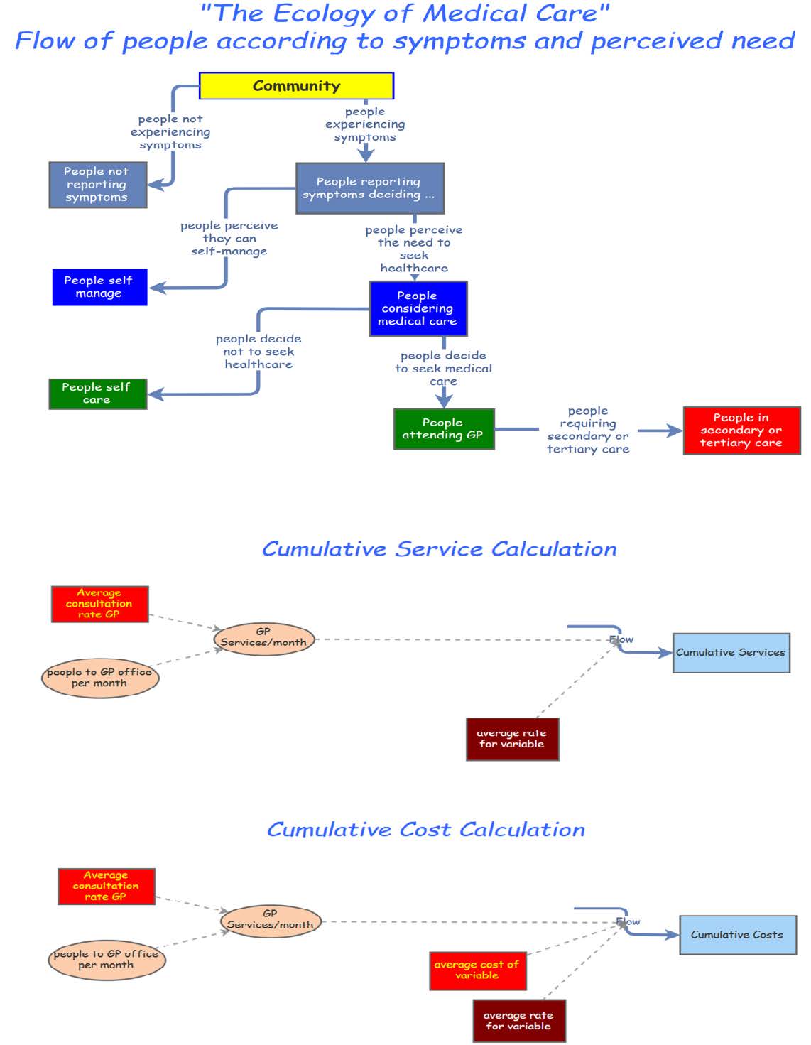
Fortmann-Roe S (2014) Insight Maker: A general-purpose tool for web-based modeling & simulation. Simulation Model Practice Theory 47: 28-45. doi: 10.1016/j.simpat.2014.03.013
![]() |
[7] |
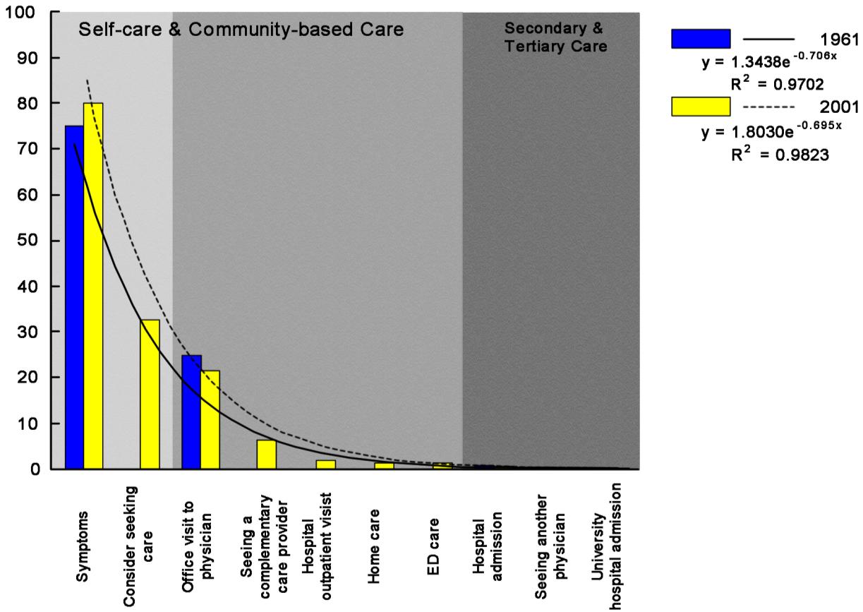
White K, Williams F, Greenberg B (1961) The Ecology of Medical Care. N Engl J Med 265: 885-892. doi: 10.1056/NEJM196111022651805
![]() |
[8] |
Green L, Fryer G, Yawn B, et al. (2001) The Ecology of Medical Care Revisited. N Engl J Med 344: 2021-2025. doi: 10.1056/NEJM200106283442611
![]() |
[9] |
Johansen ME, Kircher SM, Huerta TR (2016) Reexamining the Ecology of Medical Care. N Engl J Med 374: 495-496. doi: 10.1056/NEJMc1506109
![]() |
[10] | Sturmberg JP, O'Halloran DM, Martin CM (2014) Health Care Reform—The Need for a Complex Adaptive Systems Approach. In: Sturmberg JP, Martin CM, editors. Handbook of Systems and Complexity in Health. New York: Springer; p. 827-853. |
[11] | Britt H, Miller GC, Henderson J, et al. (2013) General practice activity in Australia 2012–13. Sydney: 2013 Contract No.: General practice series no.33. |
[12] | Australian Institute of Health and Welfare. (2014) Australian hospital statistics 2012–13. Canberra: Australian Institute of Health and Welfare, Cat. No. HSE 145. |
[13] | Australian Institute of Health and Welfare. (2014) Australian hospital statistics 2012–13. Emergency department care. Canberra: Australian Institute of Health and Welfare, Cat. No. HSE 142. |
[14] | Medicare Australia. (http://wwwmedicareaustraliagovau/cgi-bin/brokerexe?_PROGRAM=sasmbs_group_standard_reportsas&_SERVICE=default&DRILL=on&_DEBUG=0&GROUP=1&VAR=services&STAT=count&RPT_FMT=by+state&PTYPE=finyear&START_DT=201207&END_DT=201306). |
[15] | Department of Health. http://wwwhumanservicesgovau/corporate/statistical-information-and-data/pharmaceutical-benefits-schedule-statistics/. |
[16] |
Nissen SE (2015) Reforming the continuing medical education system. JAMA 313: 1813-1814. doi: 10.1001/jama.2015.4138
![]() |
[17] | Alper J, Geller A (2015) How modeling can inform strategies to improve population health: Workshop summary. National Academies of Sciences, Engineering, and Medicine. Washington, DC: The National Academies Press. |
[18] |
Howie J, Heaney D, Maxwell M, et al. (1999) Quality at general practice consultations: cross sectional survey. Br Med J 319: 738-743. doi: 10.1136/bmj.319.7212.738
![]() |
[19] | Howie JGR, Porter AMD, Heaney DJ, et al. (1991) Long to short consultation ratio: a proxy measure of quality of care for general practice. Br J Gen Pract 41: 48-54. |
[20] | Freeman G, Horder J, Howie J, et al. (2002) Evolving general practice consultation in Britain: issues of length and context. Br Med J 324: 820-822. |
[21] |
Hart JT (1998) Expectations of health care: promoted, managed or shared? Health Expect 1: 3-13. doi: 10.1046/j.1369-6513.1998.00001.x
![]() |
[22] |
Hjortdahl P, Borchgrevink CF (1991) Continuity of care—influence of general practitioners' knowledge about their patients on use of resources in consultations. Br Med J 303: 1181-1184. doi: 10.1136/bmj.303.6811.1181
![]() |
[23] |
Hjortdahl P (1992) The Influence of General Practitioners' Knowledge about their Patients on the Clinical Decision-Making Process. Scand J Prim Health Care 10: 290-294. doi: 10.3109/02813439209014076
![]() |
[24] |
Reeve J, Blakeman T, Freeman G, et al. (2013) Generalist solutions to complex problems: generating practice-based evidence—the example of managing multi-morbidity. BMC Family Practice 14: 112. doi: 10.1186/1471-2296-14-112
![]() |
[25] |
Stange KC, Ferrer RL (2009) The Paradox of Primary Care. Ann Fam Med 7: 293-299. doi: 10.1370/afm.1023
![]() |
[26] | Martin CM, Grady D, Deaconking S, et al. (2014) Complex adaptive chronic care—typologies of patient journey: a case study. J Eval Clin Pract 17: 520-524. |
[27] | Sturmberg JP, O’Halloran DM, Martin CM (2010) People at the centre of complex adaptive health systems reform. Med J Aust 193: 474-478. |
[28] | Heifetz R (1994) Leadership Without Easy Answers. Cambridge, Ma: Harvard University Press. |
1. | Martin Heida, Benedikt Jahnel, Anh Duc Vu, An ergodic and isotropic zero-conductance model with arbitrarily strong local connectivity, 2024, 29, 1083-589X, 10.1214/24-ECP633 |