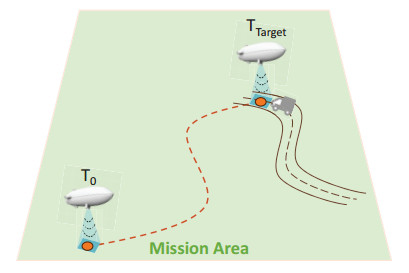
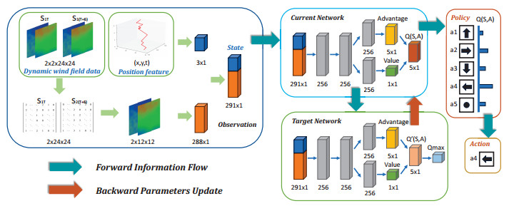
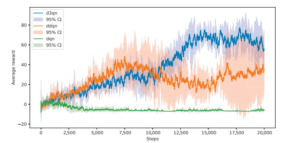
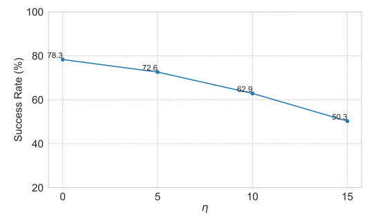
Large-scale movement over a fixed time is one of the unique tasks of stratospheric airships. In practical applications, stratospheric airships often need to arrive at the designated location on time when performing tasks such as monitoring and detection. Due to the large wind resistance and low ship speed, stratospheric airships are easily affected by wind during long-distance movement. Therefore, determining how to ensure that the airship arrives at the designated location within the target time under the influence of dynamic wind fields is an urgent problem to be solved. This paper proposes an innovative solution. Based on the dueling double deep Q-network (D3QN) architecture, a trajectory planning algorithm (named FTD3) for fixed-time large-scale maneuvers was constructed. By preprocessing the wind field data and reducing the amount of input data, all information about the future wind field can be retained without introducing the instantaneous wind field. A new reward function was designed to incorporate time and distance constraints into the same dimension through time–distance mapping. Comparative experiments with other architectures showed that in the test set verification, the success rate of FTD3 reached 78.3%, compared to 47.7% for the double deep Q-network (DDQN)-based algorithm. Compared to other algorithms, FTD3 could avoid overfitting problems with the same training step size and yielded good results in uncertain wind fields. In summary, FTD3 provides an effective solution for the trajectory planning of stratospheric airships for scheduled and large-scale movement in dynamic wind fields.
Citation: Qinchuan Luo, Kangwen Sun, Tian Chen, Ming Zhu, Zewei Zheng. Stratospheric airship fixed-time trajectory planning based on reinforcement learning[J]. Electronic Research Archive, 2025, 33(4): 1946-1967. doi: 10.3934/era.2025087
Large-scale movement over a fixed time is one of the unique tasks of stratospheric airships. In practical applications, stratospheric airships often need to arrive at the designated location on time when performing tasks such as monitoring and detection. Due to the large wind resistance and low ship speed, stratospheric airships are easily affected by wind during long-distance movement. Therefore, determining how to ensure that the airship arrives at the designated location within the target time under the influence of dynamic wind fields is an urgent problem to be solved. This paper proposes an innovative solution. Based on the dueling double deep Q-network (D3QN) architecture, a trajectory planning algorithm (named FTD3) for fixed-time large-scale maneuvers was constructed. By preprocessing the wind field data and reducing the amount of input data, all information about the future wind field can be retained without introducing the instantaneous wind field. A new reward function was designed to incorporate time and distance constraints into the same dimension through time–distance mapping. Comparative experiments with other architectures showed that in the test set verification, the success rate of FTD3 reached 78.3%, compared to 47.7% for the double deep Q-network (DDQN)-based algorithm. Compared to other algorithms, FTD3 could avoid overfitting problems with the same training step size and yielded good results in uncertain wind fields. In summary, FTD3 provides an effective solution for the trajectory planning of stratospheric airships for scheduled and large-scale movement in dynamic wind fields.

| [1] |
J. Gonzalo, D. Domínguez, A. García-Gutiérrez, A. Escapa, On the development of a parametric aerodynamic model of a stratospheric airship, Aerosp. Sci. Technol., 107 (2020), 106316. https://doi.org/10.1016/j.ast.2020.106316 doi: 10.1016/j.ast.2020.106316

|
| [2] |
Z. Zuo, J. Song, Z. Zheng, Q. L. Han, A survey on modelling, control and challenges of stratospheric airships, Control Eng. Pract., 119 (2022), 104979. https://doi.org/10.1016/j.conengprac.2021.104979 doi: 10.1016/j.conengprac.2021.104979
|
| [3] |
R. Chai, H. Niu, J. Carrasco, F. Arvin, H. Yin, B. Lennox, Design and experimental validation of deep reinforcement learning-based fast trajectory planning and control for mobile robot in unknown environment, IEEE Trans. Neural Networks Learn. Syst., 35 (2022), 5778–5792. https://doi.org/10.1109/TNNLS.2022.3209154 doi: 10.1109/TNNLS.2022.3209154
|
| [4] |
Y. Yang, X. Xiong, Y. Yan, Uav formation trajectory planning algorithms: A review, Drones, 7 (2023), 62. https://doi.org/10.3390/drones7010062 doi: 10.3390/drones7010062
|
| [5] |
Y. Li, B. Li, W. Yu, S. Zhu, X. Guan, Cooperative localization based multi-auv trajectory planning for target approaching in anchor-free environments, IEEE Trans. Veh. Technol., 71 (2021), 3092–3107. https://doi.org/10.1109/TVT.2021.3137171 doi: 10.1109/TVT.2021.3137171
|
| [6] |
E. Zhang, R. Zhang, N. Masoud, Predictive trajectory planning for autonomous vehicles at intersections using reinforcement learning, Transp. Res. Part C Emerging Technol., 149 (2023), 104063. https://doi.org/10.1016/j.trc.2023.104063 doi: 10.1016/j.trc.2023.104063
|
| [7] |
L. Liu, Q. Shan, Q. Xu, Usvs path planning for maritime search and rescue based on pos-dqn: Probability of success-deep q-network, J. Mar. Sci. Eng., 12 (2024), 1158. https://doi.org/10.3390/jmse12071158 doi: 10.3390/jmse12071158
|
| [8] |
C. Dong, Y. Zhang, Z. Jia, Y. Liao, L. Zhang, Q. Wu, Three-dimension collision-free trajectory planning of uavs based on ads-b information in low-altitude urban airspace, Chin. J. Aeronaut., 38 (2025), 103170. https://doi.org/10.1016/j.cja.2024.08.001 doi: 10.1016/j.cja.2024.08.001
|
| [9] |
X. Wu, Y. Yang, Y. Sun, Y. Xie, X. Song, B. Huang, Dynamic regional splitting planning of remote sensing satellite swarm using parallel genetic pso algorithm, Acta Astronaut., 204 (2023), 531–551. https://doi.org/10.1016/j.actaastro.2022.09.020 doi: 10.1016/j.actaastro.2022.09.020
|
| [10] |
J. Kikuchi, R. Nakamura, S. Ueda, Comparison of transfer trajectory to nrho and operation plan for logistics resupply mission to gateway, Acta Astronaut., 223 (2024), 577–584. https://doi.org/10.1016/j.actaastro.2024.07.038 doi: 10.1016/j.actaastro.2024.07.038
|
| [11] |
J. Fan, X. Chen, X. Liang, Uav trajectory planning based on bi-directional apf-rrt* algorithm with goal-biased, Expert Syst. Appl., 213 (2023), 119137. https://doi.org/10.1016/j.eswa.2022.119137 doi: 10.1016/j.eswa.2022.119137
|
| [12] |
Y. Zhang, K. Yang, T. Chen, Z. Zheng, M. Zhu, Integration of path planning and following control for the stratospheric airship with forecasted wind field data, ISA Trans., 143 (2023), 115–130. https://doi.org/10.1016/j.isatra.2023.08.026 doi: 10.1016/j.isatra.2023.08.026
|
| [13] |
Q. C. Luo, K. W. Sun, T. Chen, Y. f. Zhang, Z. W. Zheng, Trajectory planning of stratospheric airship for station-keeping mission based on improved rapidly exploring random tree, Adv. Space Res., 73 (2024), 992–1005. https://doi.org/10.1016/j.asr.2023.10.002 doi: 10.1016/j.asr.2023.10.002
|
| [14] | A. Gasparetto, P. Boscariol, A. Lanzutti, R. Vidoni, Path planning and trajectory planning algorithms: A general overview, in Motion and Operation Planning of Robotic Systems. Mechanisms and Machine Science, Springer, Cham, 29 (2015), 3–27. https://doi.org/10.1007/978-3-319-14705-5_1 |
| [15] |
H. Jin, R. Xu, P. Cui, S. Zhu, H. Jiang, F. Zhou, Heuristic search via graphical structure in temporal interval-based planning for deep space exploration, Acta Astronaut., 166 (2020), 400–412. https://doi.org/10.1016/j.actaastro.2019.10.002 doi: 10.1016/j.actaastro.2019.10.002
|
| [16] |
R. Ueda, L. Tonouchi, T. Ikebe, Y. Hayashibara, Implementation of brute-force value iteration for mobile robot path planning and obstacle bypassing, J. Rob. Mechatron., 35 (2023), 1489–1502. https://doi.org/10.20965/jrm.2023.p1489 doi: 10.20965/jrm.2023.p1489
|
| [17] | P. Gupta, D. Isele, D. Lee, S. Bae, Interaction-aware trajectory planning for autonomous vehicles with analytic integration of neural networks into model predictive control, in 2023 IEEE International Conference on Robotics and Automation (ICRA), IEEE, (2023), 7794–7800. https://doi.org/10.1109/ICRA48891.2023.10160890 |
| [18] |
Y. Qin, Z. Zhang, X. Li, W. Huangfu, H. Zhang, Deep reinforcement learning based resource allocation and trajectory planning in integrated sensing and communications uav network, IEEE Trans. Wireless Commun., 22 (2023), 8158–8169. https://doi.org/10.1109/TWC.2023.3260304 doi: 10.1109/TWC.2023.3260304
|
| [19] |
F. Wang, H. Zhang, S. Du, M. Hua, G. Zhong, C-sppo: A deep reinforcement learning framework for large-scale dynamic logistics uav routing problem, Chin. J. Aeronaut., 38 (2025), 103229. https://doi.org/10.1016/j.cja.2024.09.005 doi: 10.1016/j.cja.2024.09.005
|
| [20] |
C. Wu, W. Yu, G. Li, W. Liao, Deep reinforcement learning with dynamic window approach based collision avoidance path planning for maritime autonomous surface ships, Ocean Eng., 284 (2023), 115208. https://doi.org/10.1016/j.oceaneng.2023.115208 doi: 10.1016/j.oceaneng.2023.115208
|
| [21] |
X. Zheng, J. Cao, B. Zhang, Y. Zhang, W. Chen, Y. Dai, et al., Path planning of prm based on artificial potential field in radiation environments, Ann. Nucl. Energy, 208 (2024), 110776. https://doi.org/10.1016/j.anucene.2024.110776 doi: 10.1016/j.anucene.2024.110776
|
| [22] |
L. Qi, X. Yang, F. Bai, X. Deng, Y. Pan, Stratospheric airship trajectory planning in wind field using deep reinforcement learning, Adv. Space Res., 75 (2025), 620–634. https://doi.org/10.1016/j.asr.2024.08.057 doi: 10.1016/j.asr.2024.08.057
|
| [23] | Y. Wang, B. Zheng, W. Lou, L. Sun, C. Lv, Trajectory planning of stratosphere airship in wind-cloud environment based on soft actor-critic, in 2024 IEEE International Conference on Artificial Intelligence in Engineering and Technology (IICAIET), IEEE, (2024), 401–406. https://doi.org/10.1109/IICAIET62352.2024.10730558 |
| [24] |
S. Liu, S. Zhou, J. Miao, H. Shang, Y. Cui, Y. Lu, Autonomous trajectory planning method for stratospheric airship regional station-keeping based on deep reinforcement learning, Aerospace, 11 (2024), 753. https://doi.org/10.3390/aerospace11090753 doi: 10.3390/aerospace11090753
|
| [25] |
M. Xi, J. Yang, J. Wen, H. Liu, Y. Li, H. H. Song, Comprehensive ocean information-enabled auv path planning via reinforcement learning, IEEE Internet Things J., 9 (2022), 17440–17451. https://doi.org/10.1109/JIOT.2021.3137742 doi: 10.1109/JIOT.2021.3137742
|
| [26] |
A. G. S. Junior, D. H. Santos, A. P. F. Negreiros, J. M. V. B. S. Silva, L. M. G. Gonçalves, High-level path planning for an autonomous sailboat robot using q-learning, Sensors, 20 (2020), 1550. https://doi.org/10.3390/s20061550 doi: 10.3390/s20061550
|
| [27] |
S. Woo, J. Park, J. Park, L. Manuel, Wind field-based short-term turbine response forecasting by stacked dilated convolutional LSTMs, IEEE Trans. Sustainable Energy, 11 (2019), 2294–2304. https://doi.org/10.1109/TSTE.2019.2954107 doi: 10.1109/TSTE.2019.2954107
|
Figures(11) / Tables(3)
Qinchuan Luo, Kangwen Sun, Tian Chen, Ming Zhu, Zewei Zheng. Stratospheric airship fixed-time trajectory planning based on reinforcement learning[J]. Electronic Research Archive, 2025, 33(4): 1946-1967. doi: 10.3934/era.2025087


 DownLoad: