Analytical model of solar energy storage using non—Newtonian Fluid in a saturated porous media in fully developed region: carboxymethyl cellulose (CMC) and graphite model

Eman S. Maayah; Hamzeh M. Duwairi; Banan Maayah; Eman S. Maayah; Hamzeh M. Duwairi; Banan Maayah

doi:10.3934/energy.2021012

AIMS Energy

2021, Volume 9, Issue 2: 213-237. doi: 10.3934/energy.2021012

Previous Article Next Article

Research article

Analytical model of solar energy storage using non—Newtonian Fluid in a saturated porous media in fully developed region: carboxymethyl cellulose (CMC) and graphite model

1.
Mechanical Engineering Department, school of Engineering, The University of Jordan, Amman 11942, Jordan
2.
Mathematic Department, school of Science, The University of Jordan, Amman 11942, Jordan

Received: 14 October 2020 Accepted: 08 January 2021 Published: 18 January 2021

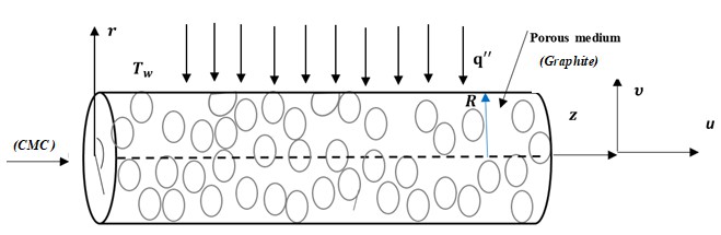
Thermal energy storage systems are used mainly in buildings and industrial processes. In this study, solar energy storage by using a circular conduit filled with porous media that is saturated by a non-Newtonian fluid at constant heat flux was represented.

The fully developed region was studied by solving the equations analytically, the non-Newtonian fluid parameters used in this model are carboxymethyl cellulose (CMC) properties. In addition, graphite was used as porous media. The heat flux data for Amman city was used in the equations in this study.

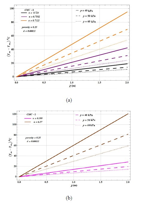
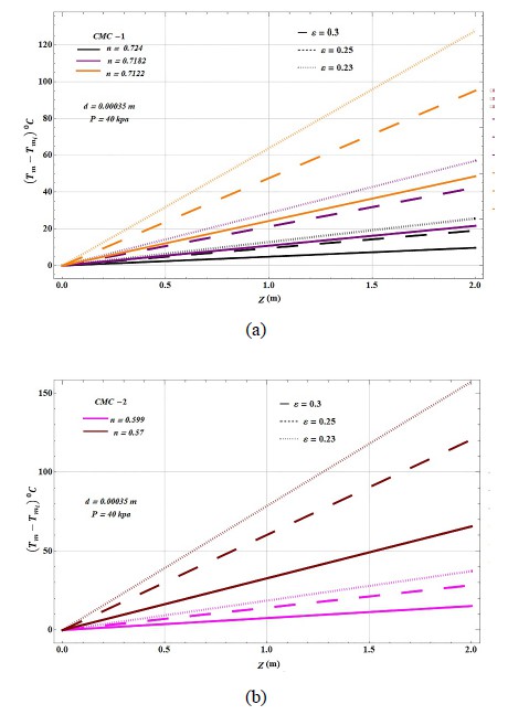
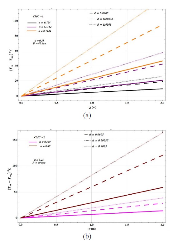
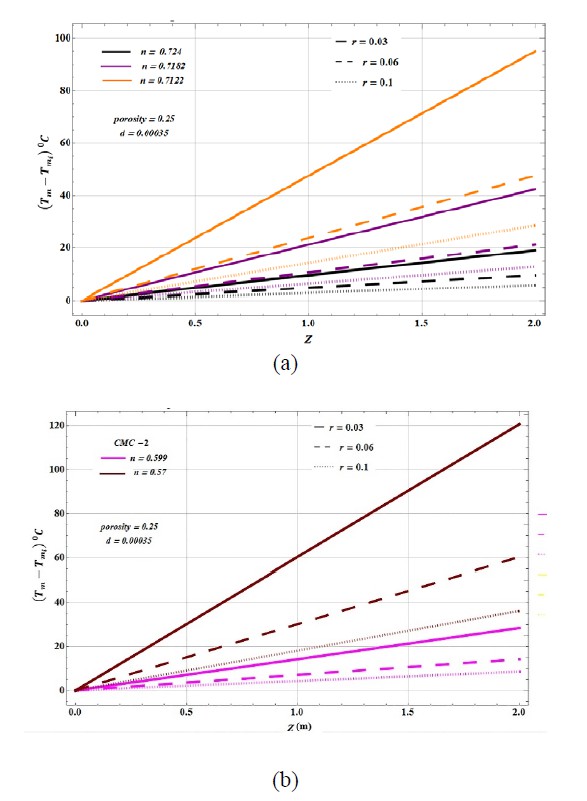
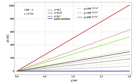
The effect of Porosity and particle diameter and pressure on the performance of the model were discussed and sketched. As a result, the temperature of storage filled with CMC fluid is better than water in porous media. It is found that the power index of the fluid, porosity, particle diameter, pressure drop, and conduit radius effect inversely the temperature in energy storage.

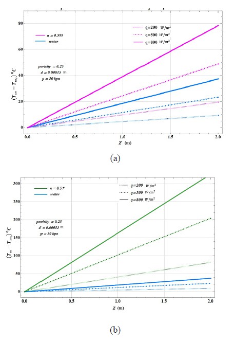
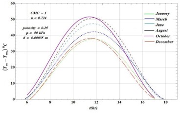
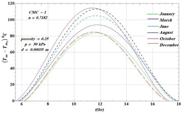
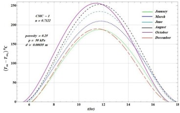
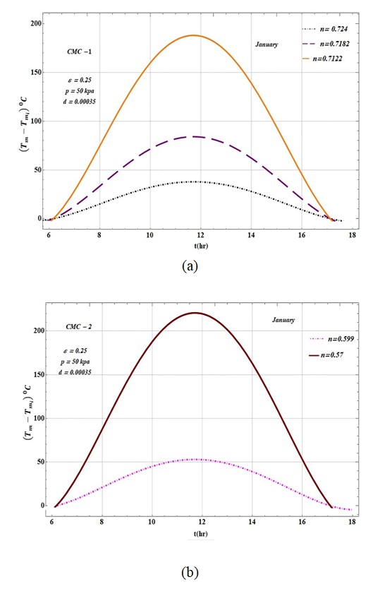
In January, the temperature variation in conduit at the same conditions reach for CMC-1 to 35 ℃ for n = 0.724 and to 85 ℃ for n = 0.7182 and to 190 ℃ for n = 0.7122.

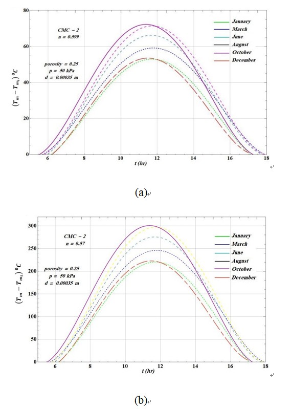
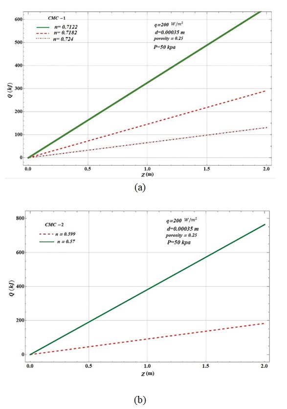
CMC-2 has a higher consistency index at the same concentration which means higher viscosity and less power index than CMC-1 so the temperature variation in conduit reaches 50 ℃ for n = 0.599 and 200 ℃ for n = 0.57. The stored energy of CMC-1 for n = 0.724, n = 0.7182, and n = 0.7122 is approximately 120 kJ, 300 kJ, and more than 600 kJ respectively, and the stored energy of CMC-2 n = 0.599 and n = 0.57 is 200 kJ and approach to 800 kJ at the same conditions and conduit.
- solar energy storage,
- Non-Newtonian,
- porous media,
- fully developed,
- CMC
Citation: Eman S. Maayah, Hamzeh M. Duwairi, Banan Maayah. Analytical model of solar energy storage using non—Newtonian Fluid in a saturated porous media in fully developed region: carboxymethyl cellulose (CMC) and graphite model[J]. AIMS Energy, 2021, 9(2): 213-237. doi: 10.3934/energy.2021012

Related Papers:

Abstract

Thermal energy storage systems are used mainly in buildings and industrial processes. In this study, solar energy storage by using a circular conduit filled with porous media that is saturated by a non-Newtonian fluid at constant heat flux was represented.

The fully developed region was studied by solving the equations analytically, the non-Newtonian fluid parameters used in this model are carboxymethyl cellulose (CMC) properties. In addition, graphite was used as porous media. The heat flux data for Amman city was used in the equations in this study.

The effect of Porosity and particle diameter and pressure on the performance of the model were discussed and sketched. As a result, the temperature of storage filled with CMC fluid is better than water in porous media. It is found that the power index of the fluid, porosity, particle diameter, pressure drop, and conduit radius effect inversely the temperature in energy storage.

In January, the temperature variation in conduit at the same conditions reach for CMC-1 to 35 ℃ for n = 0.724 and to 85 ℃ for n = 0.7182 and to 190 ℃ for n = 0.7122.

CMC-2 has a higher consistency index at the same concentration which means higher viscosity and less power index than CMC-1 so the temperature variation in conduit reaches 50 ℃ for n = 0.599 and 200 ℃ for n = 0.57. The stored energy of CMC-1 for n = 0.724, n = 0.7182, and n = 0.7122 is approximately 120 kJ, 300 kJ, and more than 600 kJ respectively, and the stored energy of CMC-2 n = 0.599 and n = 0.57 is 200 kJ and approach to 800 kJ at the same conditions and conduit.

References

[1]	Macdonald I, Gaigher I, Gaigher R, et al. (2003) Electrical Energy Storage, Geneva, Switzerland. Available from: https://basecamp.iec.ch/download/iec-white-paper-electrical-energy-storage/.
[2]	Marinet M, Tardu S (2009) Convective Heat Transfer. UK: ISTE Ltd, USA: John Wiley & Sons, Inc.
[3]	Dhifaoui B, Ben Jabrallah S, Belghith A, et al. (2007) Experimental study of the dynamic behaviour of a porous medium submitted to a wall heat flux in view of thermal energy storage by sensible heat. Int J Therm Sci 46: 1056-1063. doi: 10.1016/j.ijthermalsci.2006.11.014
[4]	Hänchen M, Brückner S, Steinfeld A (2011) High-temperature thermal storage using a packed bed of rocks—Heat transfer analysis and experimental validation. Appl Therm Eng 31: 1798-1806. doi: 10.1016/j.applthermaleng.2010.10.034
[5]	Kim J, Jeong E, Lee Y (2015) Preparation and characterization of graphite foams. J Ind Eng Chem 32: 1-33. doi: 10.1016/j.jiec.2015.08.004
[6]	Wu Z, Zhao C (2011) Experimental investigations of porous materials in high temperature thermal energy storage systems. Sol Energy 85: 1371-1380. doi: 10.1016/j.solener.2011.03.021
[7]	Chamkha A, Abbasbandy S, Rashadm A (2014) Non-Darcy natural convection flow for non-Newtonian nanofluid over cone saturated in porous medium with uniform heat and volume fraction fluxes. Int J Numer Methods Heat Fluid Flow 24: 422-437.
[8]	Karaipekli A, Biçer A, Sarı A, et al. (2017) Thermal characteristics of expanded perlite/paraffin composite phase change material with enhanced thermal conductivity using carbon nanotubes. Energy Convers Manag 134: 373-381. doi: 10.1016/j.enconman.2016.12.053
[9]	Mohammed M, Mohammed A (2009) Effect of type and concentration of different water soluble polymer solutions on rheological properties. Nahrain Univ Coll Eng J 12: 26-37.
[10]	Doerr M, Frommherz M (2002) Graphite (C)—Classifications, properties & applications. Available from: https://www.azom.com/article.aspx?ArticleID=1630.
[11]	Sanchez-Coronado J, Chung D (2003) Thermomechanical behavior of a graphite foam. Carbon 41: 1175-1180. doi: 10.1016/S0008-6223(03)00025-3
[12]	Oosthuizen P, Naylor D (1999) Introduction to convective heat transfer analysis. New York: WCB/McGraw Hill.
[13]	Muzychka Y, Yovanovich M (2014) Convective heat transfer, Handbook of Fluid Dynamics, CRC Press, (In Press).
[14]	Besson U (2012) The history of the cooling law: When the search for simplicity can be an obstacle. Sci Educ 21: 1085-1110. doi: 10.1007/s11191-010-9324-1
[15]	Christopher R, Middleman S (1965) Power-law flow through a packed tube. Ind Eng Chem Fundam 4: 422-426. doi: 10.1021/i160016a011
[16]	Shenoy A (2017) Heat transfer to non‐newtonian fluids. United States: Wiley-VCH, 3.
[17]	JRC Photovoltaic Geographical Information System (PVGIS)—European Commission. Available from: https://re.jrc.ec.europa.eu/pvg_tools/en/tools.html (accessed Nov. 13, 2019).
[18]	Kuravi S, Trahan J, Goswami D, et al. (2013) Thermal energy storage technologies and systems for concentrating solar power plants. Prog Energy Combust Sci 39: 285-319. doi: 10.1016/j.pecs.2013.02.001

Reader Comments

Your name:*

Email:*
© 2021 the Author(s), licensee AIMS Press. This is an open access article distributed under the terms of the Creative Commons Attribution License (http://creativecommons.org/licenses/by/4.0)