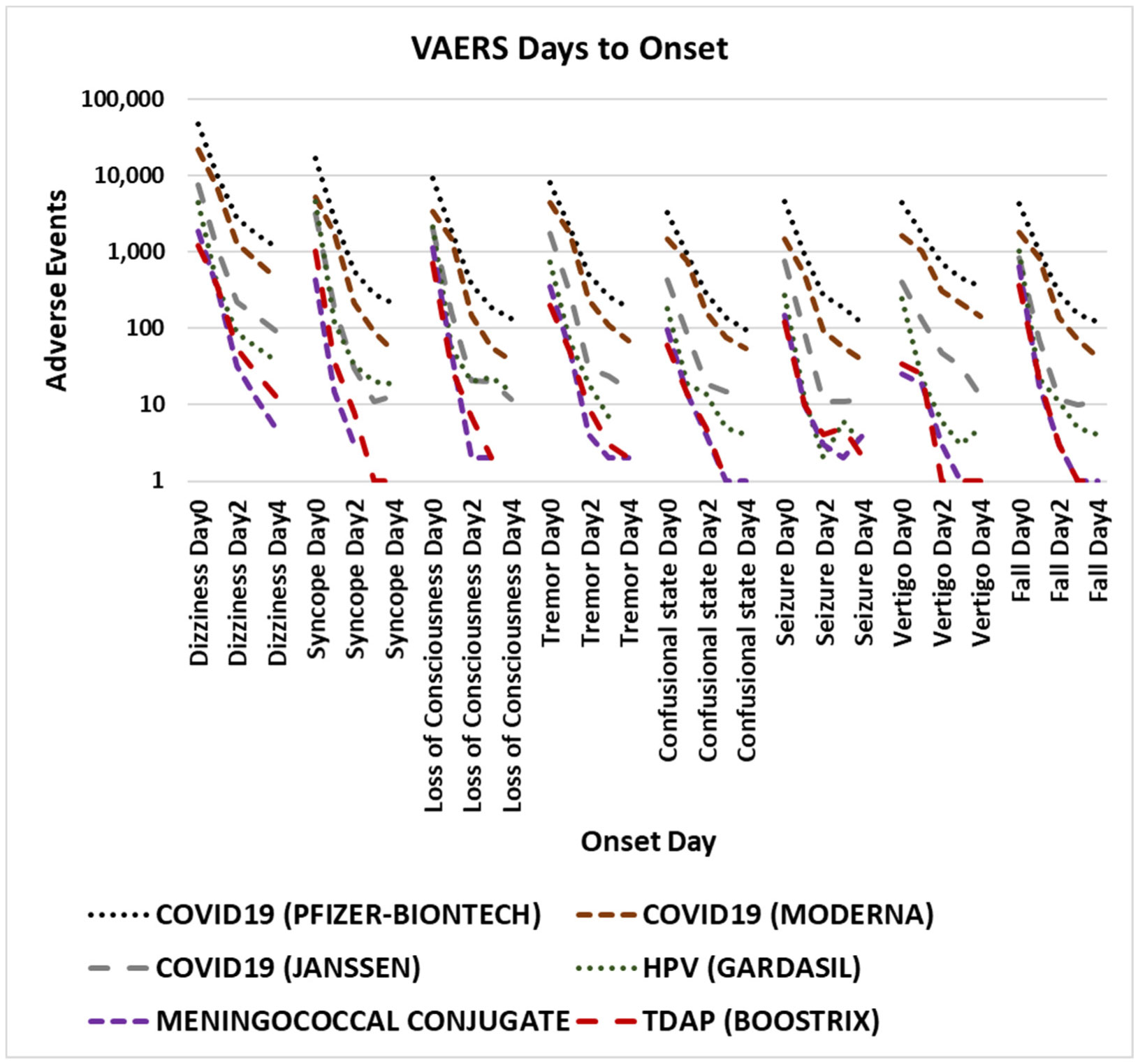
Some individuals experience dizziness, syncope (temporary loss of consciousness caused by a fall in blood pressure), seizure, and similar rare adverse events after vaccination. Sudden impacts to alertness, consciousness, ability to talk, vision, or balance may pose rare risks for some vaccinees for a few days post vaccination. Herein, the Vaccine Adverse Event Reporting System (VAERS) database is examined for relevant adverse events. These adverse events exhibit a consistent pattern of onset soon after vaccination consistent with other reported reactogenicity adverse events. The onset of these adverse events soon after vaccination provides supportive evidence to reject the hypothesis that the majority of these adverse events represent background occurrences unrelated to vaccination. The immediate onset timing of these adverse events represent a pattern that warrants further study. The observed onset pattern for multiple unrelated vaccines are consistent with the possible etiology of innate immune responses to vaccination as causative for these observed adverse events. Cautionary avoidance of some activities immediately following vaccination may reduce accidental injuries.
Citation: Darrell O. Ricke. Rare dizziness, syncope, loss of consciousness, seizure, and risk of falling after vaccination[J]. AIMS Allergy and Immunology, 2023, 7(2): 164-175. doi: 10.3934/Allergy.2023011
Some individuals experience dizziness, syncope (temporary loss of consciousness caused by a fall in blood pressure), seizure, and similar rare adverse events after vaccination. Sudden impacts to alertness, consciousness, ability to talk, vision, or balance may pose rare risks for some vaccinees for a few days post vaccination. Herein, the Vaccine Adverse Event Reporting System (VAERS) database is examined for relevant adverse events. These adverse events exhibit a consistent pattern of onset soon after vaccination consistent with other reported reactogenicity adverse events. The onset of these adverse events soon after vaccination provides supportive evidence to reject the hypothesis that the majority of these adverse events represent background occurrences unrelated to vaccination. The immediate onset timing of these adverse events represent a pattern that warrants further study. The observed onset pattern for multiple unrelated vaccines are consistent with the possible etiology of innate immune responses to vaccination as causative for these observed adverse events. Cautionary avoidance of some activities immediately following vaccination may reduce accidental injuries.
coronavirus disease 2019
human papillomavirus
messenger ribonucleic acid
severe acute respiratory syndrome coronavirus 2
tetanus, diphtheria, and pertussis
Vaccine Adverse Event Reporting System

| [1] |
Ricke DO (2022) Etiology model for many vaccination adverse reactions, including SARS-CoV-2 spike vaccines. AIMS Allergy Immunol 6: 200-215. https://doi.org/10.3934/Allergy.2022015 
|
| [2] |
Okuyama M, Morino S, Tanaka K, et al. (2022) Vasovagal reactions after COVID-19 vaccination in Japan. Vaccine 40: 5997-6000. https://doi.org/10.1016/j.vaccine.2022.08.056
|
| [3] |
Tri A, Mills K, Nilsen K (2022) Pediatric COVID-19 vaccination: A description of adverse events or reactions reported in Kansans aged 6 to 17. Kans J Med 15: 390-393. https://doi.org/10.17161/kjm.vol15.18431
|
| [4] |
Gallo AT, Scanlon L, Clifford J, et al. (2022) Immediate adverse events following COVID-19 vaccination in Australian pharmacies: A retrospective review. Vaccines 10: 2041. https://doi.org/10.3390/vaccines10122041
|
| [5] |
Takase B, Hisada T, Masaki N, et al. (2022) Frequency of vaccine-associated syncope after COVID-19 vaccination in adolescents. J Arrhythm 38: 448-450. https://doi.org/10.1002/joa3.12721
|
| [6] |
Takase B, Hayashi K, Takei S, et al. (2022) Delayed vasovagal reaction with reflex syncope following COVID-19 vaccination. Internal Med 61: 2167-2170. https://doi.org/10.2169/internalmedicine.9318-21
|
| [7] |
Almohaya AM, Alsubie H, Alqarni B, et al. (2022) Acute unsolicited adverse events following BNT162b2 vaccine in Saudi Arabia, a real-world data. Vaccine 40: 477-482. https://doi.org/10.1016/j.vaccine.2021.12.001
|
| [8] |
Ab Rahman N, Lim MT, Lee FY, et al. (2022) Risk of serious adverse events after the BNT162b2, CoronaVac, and ChAdOx1 vaccines in Malaysia: A self-controlled case series study. Vaccine 40: 4394-4402. https://doi.org/10.1016/j.vaccine.2022.05.075
|
| [9] |
Núñez I, García-Grimshaw M, Valencia CYC, et al. (2022) Seizures following COVID-19 vaccination in Mexico: A nationwide observational study. Epilepsia 63: e144-e149. https://doi.org/10.1111/epi.17390
|
| [10] |
Martinez-Fernandez I, Sanchez-Larsen A, Gonzalez-Villar E, et al. (2022) Observational retrospective analysis of vaccination against SARS-CoV-2 and seizures: VACCI-COVID registry. Epilepsy Behav 134: 108808. https://doi.org/10.1016/j.yebeh.2022.108808
|
| [11] |
Hviid A (2011) Measles-mumps-rubella-varicella combination vaccine increases risk of febrile seizure. J Pediatr 158: 170. https://doi.org/10.1016/j.jpeds.2010.09.075
|
| [12] |
Comas-Basté O, Sánchez-Pérez S, Veciana-Nogués MT, et al. (2020) Histamine intolerance: The current state of the art. Biomolecules 10: 1181. https://doi.org/10.3390/biom10081181
|
| [13] |
Kovacova-Hanuskova E, Buday T, Gavliakova S, et al. (2015) Histamine, histamine intoxication and intolerance. Allergol Immunopathol 43: 498-506. https://doi.org/10.1016/j.aller.2015.05.001
|
| [14] |
Jennings SV, Slee VM, Finnerty CC, et al. (2021) Symptoms of mast cell activation: The patient perspective. Ann Allerg Asthma Im 127: 407-409. https://doi.org/10.1016/j.anai.2021.07.004
|
| [15] |
Nguyen SMT, Rupprecht CP, Haque A, et al. (2021) Mechanisms governing anaphylaxis: Inflammatory cells, mediators, endothelial gap junctions and beyond. Int J Mol Sci 22: 7785. https://doi.org/10.3390/ijms22157785
|
| [16] | Ricke DO (2022) Etiology model for elevated histamine levels driving high reactogenicity vaccines (including COVID-19) associated menstrual adverse events. J Infect Dis Ther 10: 002. Available from: https://www.omicsonline.org/open-access/etiology-model-for-elevated-histamine-levels-driving-high-reactogenicity-vaccines-including-covid19-associated-menstrual-adverse-e-120159.html. |
| [17] |
Ricke DO (2022) Vaccines associated cardiac adverse events, including SARS-CoV-2 myocarditis, elevated histamine etiology hypothesis. J Virol Viral Dis 2: 1-11. https://doi.org/10.54289/JVVD2200108
|
| [18] |
Hrubisko M, Danis R, Huorka M, et al. (2021) Histamine intolerance—The more we know the less we know. A review. Nutrients 13: 2228. https://doi.org/10.3390/nu13072228
|
| [19] |
Kiviranta T, Tuomisto L, Airaksinen EM (1995) Histamine in cerebrospinal fluid of children with febrile convulsions. Epilepsia 36: 276-280. https://doi.org/10.1111/j.1528-1157.1995.tb00996.x
|
| [20] |
Miyata I, Saegusa H, Sakurai M (2011) Seizure-modifying potential of histamine H1 antagonists: A clinical observation. Pediatr Int 53: 706-708. https://doi.org/10.1111/j.1442-200X.2011.03328.x
|
| [21] |
Zolaly MA (2012) Histamine H1 antagonists and clinical characteristics of febrile seizures. Int J Gen Med 5: 277-281. https://doi.org/10.2147/IJGM.S29320
|
 allergy-07-02-011-s001.xlsx allergy-07-02-011-s001.xlsx |
 |


Figures(4) / Tables(2)

Darrell O. Ricke. Rare dizziness, syncope, loss of consciousness, seizure, and risk of falling after vaccination[J]. AIMS Allergy and Immunology, 2023, 7(2): 164-175. doi: 10.3934/Allergy.2023011


 DownLoad: